
Four-rotor UAV Trajectory Planning Tutorial
Introduction
This tutorial addresses a core question: Given a set of waypoints, how can a smooth, safe, and executable flight trajectory be generated? The chapters progress step by step:
| Chapter | Core Issues Addressed | Relationship with Other Chapters |
|---|---|---|
| 1. Basics of Generating Smooth Trajectory | What is “smooth”? Which mathematical tools are used to describe the trajectory? | Defines the problem framework, introduces polynomial trajectories and constraint systems |
| 2. Minimum Snap Trajectory Optimization | How to transform the “smoothest trajectory” into a solvable mathematical optimization problem? | Depends on Chapter 1 (constraint systems), constructs a QP problem |
| 3. Corridor Constraints and Time Allocation | How to ensure the trajectory does not hit obstacles? How long is each segment flown? | Depends on Chapter 2 (QP framework), adds inequality constraints and engineering details |
| 4. Closed-Form Solution for Minimum Snap | Can the optimal solution be calculated directly without an iterative solver? | Depends on Chapter 2 (QP problem), provides an efficient analytical solution method |
Relationship to control tutorials:
- The prerequisites for this tutorial are the “III. Differential flatness” section in control tutorials—it explains why minimizing snap (fourth derivative) has physical meaning (snap corresponds to control moments)
- The output (position/velocity/acceleration reference trajectory) of this tutorial serves as the input for various controllers (PID, SE(3), MPC) in control tutorials
Reading suggestions: Just follow the order 1 → 4. If you are only interested in the principles and not the actual engineering implementation details, you can skip the time allocation and normalization parts in step 3.
Planning tutorial (4 code blocks):
- Smooth trajectory foundation — 5th polynomial interpolation, P/V/A curve
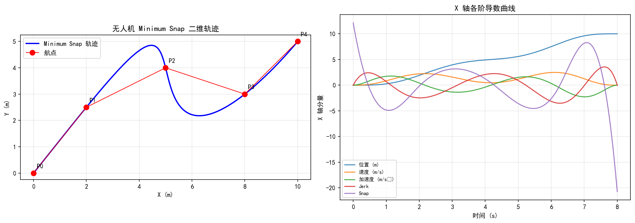
II. Minimum Snap — Minimum snap trajectory for multiple waypoints + KKT solution
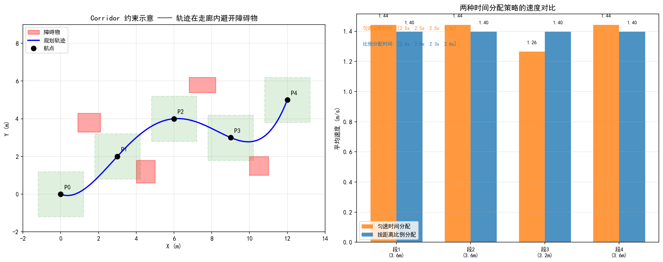
III. Corridor Constraints — Safety Passage + Obstacles + Time Allocation Policy Visualization
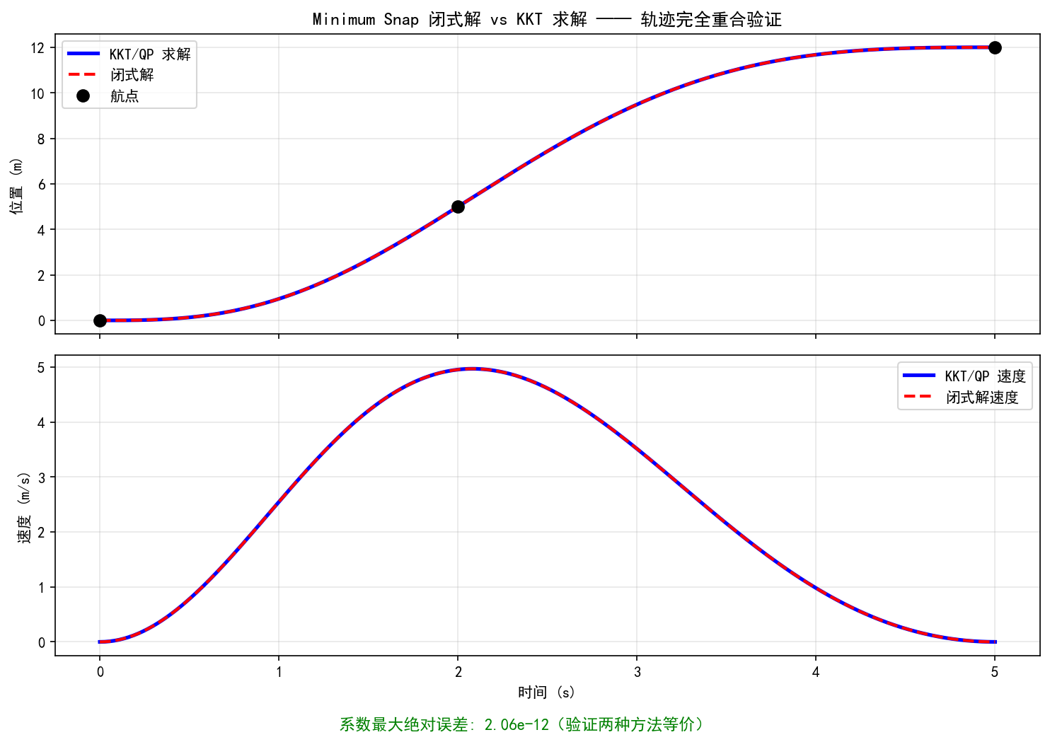
- Closed-form solution — Comparison and verification of closed-form solution and QP results
I. Basics of Smooth Trajectory Generation
1.1 Conditions for Trajectory Generation
The trajectory generation needs to meet the following conditions:
Boundary conditions:
- Starting position (determined)
- Ending position (determined)
Intermediate conditions:
- Exact position (determined, i.e., Waypoints)
Personal understanding: Waypoints are provided by front-end path planning algorithms (such as
A^* $, $RRT ,, etc.). Trajectory planning generates smooth parametrized curves based on these discrete path points.
Personal understanding: Trajectory planning is the step that follows path planning (
, , etc., which provide discrete waypoints). Path planning addresses the question of “where to go”, while trajectory planning addresses the question of “how to go” — connecting discrete path points into a smooth time-parametrized curve that satisfies kinetic constraints.
1.2 Smoothness Criteria
Personal understanding: The metric for smoothness is usually the minimization of the square integral of a derivative (i.e., the rate of change of “input”). The higher the order, the smoother the trajectory, but the higher the polynomial degree.
For a quadcopter drone, the key observation is:
- The second derivative of position (acceleration) corresponds to the thrust direction.
- The third derivative of position (jerk) corresponds to angular velocity.
- The fourth derivative of position (snap) corresponds to control torque.
Therefore, minimizing snap is equivalent to minimizing the change in control moment, ensuring smooth actuator output.
Personal understanding: The core idea of optimizing the trajectory is to optimize the square integral of the higher-order derivative of the trajectory (the smaller the rate of change, the smoother it is). Key relationships:
- If
derivatives are minimized, each segment of the polynomial is at least order ( coefficients) - Adjacent segments must ensure continuity of
derivatives - For example, minimum snap (
): each segment is a polynomial of at least 7th order, ensuring continuity of derivatives from 0 to 3
Personal understanding: Why is it a
-order polynomial? Because the integration of the square of the -order derivative to minimize is optimized over polynomial coefficients. Each segment requires constraints ( at each end), so the polynomial needs at least coefficients, i.e., order. For minimum snap ( ), each segment has at least a 7th-order polynomial (8 coefficients); in practice, 5th or 7th orders are usually chosen.
1.3 Minimizing the trajectory generation key points of Snap
- Trajectory constraints (high-order constraints): state constraints
- Continuity of the trajectory at intersections: the first derivatives at the endpoints of adjacent segments must be equal
- 4 derivatives of the trajectory: coefficient matrix and constraints
- Optimization metrics: the integral of the square of the 4th derivative of the trajectory
Special treatment at smooth straight segments:
Personal understanding: At the straight segment, the velocity direction remains constant and the acceleration is zero. However, for a smooth trajectory, the velocity direction at both ends of the straight segment (turning points) must transition smoothly, without any sudden changes in velocity or acceleration. Therefore, special handling is required for the connection between straight and curved segments.
1.4 Constraint System
Endpoint Constraints
Continuity of the
Advanced Continuity Constraints
The derivatives at the junction of adjacent segments must be equal:
Personal understanding: Taking “minimum snap” as an example, it is necessary to ensure continuity in the 0~3th derivative (position, velocity, acceleration, jerk), which requires 4 continuity constraints. These constraints ensure that there are no sudden forces or moments when the aircraft passes through points in the path.
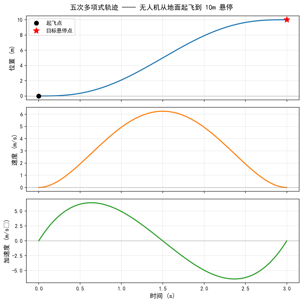
1.5 Example of a Five-Polynomial Trajectory
For minimum jerk (
Boundary conditions (6 equations, 6 parameters):
: Position , Speed , Acceleration : Position , Speed , Acceleration
Matrix solution form:
1.6 Comparison of Time Parameterization Schemes
Option 1: Relative time (each segment starts from
- Advantages: High numerical stability
Option 2: Absolute Time (using global time
- Advantages: Mathematical expressions are clear.
Personal understanding: The fatal flaw of Option 2 is that if absolute time is used, such as
seconds, then , far exceeding the precision of floating-point numbers, will cause numerical explosions. In Option 1, each segment starts at , and the range of remains within the segment duration, making the values controllable.
Personal understanding: In actual engineering, Option 1 (relative time) is usually used, as numerical stability is more important. Absolute time will cause a numerical explosion in
when is large. For example, at seconds, exceeds the precision of float by a large margin.
Python Validation
pythonimport numpy as np
import matplotlib.pyplot as plt
plt.rcParams['font.sans-serif'] = ['SimHei']  # Windows 自带黑体
plt.rcParams['axes.unicode_minus'] = False    # 解决负号显示为方框的问题
# ============================================================
# 五次多项式两点插值 —— 无人机从静止起飞到目标点
# 给定起点和终点的位置、速度、加速度,求解6x6矩阵方程得到多项式系数
# ============================================================

# --- 边界条件设置(模拟无人机垂直起飞) ---
T = 3.0          # 飞行时间 3 秒
# t=0 时刻:地面静止
pos0, vel0, acc0 = 0.0, 0.0, 0.0
# t=T 时刻:到达 10m 高度,悬停(速度和加速度均为零)
posT, velT, accT = 10.0, 0.0, 0.0

# --- 构造 6x6 约束矩阵 ---
# X(t) = p0 + p1*t + p2*t^2 + p3*t^3 + p4*t^4 + p5*t^5
A = np.array([
    [1, 0,   0,       0,         0,          0        ],   # X(0)   = pos0
    [0, 1,   0,       0,         0,          0        ],   # X'(0)  = vel0
    [0, 0,   2,       0,         0,          0        ],   # X''(0) = acc0
    [1, T,   T**2,    T**3,      T**4,       T**5     ],   # X(T)   = posT
    [0, 1,   2*T,     3*T**2,    4*T**3,     5*T**4   ],   # X'(T)  = velT
    [0, 0,   2,       6*T,       12*T**2,    20*T**3  ],   # X''(T) = accT
])
b = np.array([pos0, vel0, acc0, posT, velT, accT])

# --- 求解多项式系数 ---
coeffs = np.linalg.solve(A, b)
print("多项式系数 [p0, p1, p2, p3, p4, p5]:", np.round(coeffs, 4))

# --- 在时间轴上采样并计算 位置/速度/加速度 ---
t = np.linspace(0, T, 200)
pos = sum(coeffs[i] * t**i for i in range(6))
vel = sum(i * coeffs[i] * t**(i-1) for i in range(1, 6))
acc = sum(i * (i-1) * coeffs[i] * t**(i-2) for i in range(2, 6))

# --- 绘图 ---
fig, axes = plt.subplots(3, 1, figsize=(8, 8), sharex=True)
titles = ["位置 (m)", "速度 (m/s)", "加速度 (m/s²)"]
data = [pos, vel, acc]
colors = ["#1f77b4", "#ff7f0e", "#2ca02c"]

for ax, title, y, c in zip(axes, titles, data, colors):
    ax.plot(t, y, color=c, linewidth=2)
    ax.set_ylabel(title, fontsize=12)
    ax.grid(True, alpha=0.3)
    ax.axhline(0, color='gray', linewidth=0.5)

# 标注起点和终点
axes[0].plot(0, pos0, 'ko', markersize=8, label='起飞点')
axes[0].plot(T, posT, 'r*', markersize=12, label='目标悬停点')
axes[0].legend(fontsize=10)

axes[-1].set_xlabel("时间 (s)", fontsize=12)
fig.suptitle("五次多项式轨迹 —— 无人机从地面起飞到 10m 悬停", fontsize=13)
plt.tight_layout()
import os; os.makedirs('assets', exist_ok=True)
plt.savefig('assets/planning1.png', dpi=150, bbox_inches='tight')
plt.show()
Execution result:
II. Minimum Snap Trajectory Optimization
2.1 Mathematical Expression of Polynomial Trajectory
A
There are
Position (Stage 0):
Speed (1st order):
Acceleration (2nd order):
Jerk (3rd order, acceleration):
Snap (4th order):
Personal understanding: The
th derivative can be uniformly written as . The th element at the th position is (when ), otherwise it is 0.
2.2 Multi-segment Trajectory Representation
For the trajectory of
The parameter
Stack all segment parameters into a single vector:
2.3 Selection of Optimization Objectives
Different optimization objectives correspond to different smoothness metrics:
| Optimization Target | Expression | Meaning | Minimum Polynomial Order |
|---|---|---|---|
| Minimum Snap | Minimize torque change | 7th order | |
| Minimum Jerk | Minimize angular velocity change | 5th order | |
| Minimum Acce | Minimize acceleration | 3rd order |
Personal understanding: Generally, minimizing speed or position is not chosen, because minimizing lower-order derivatives makes the trajectory too “lazy” (tending to remain still), losing its practical significance. Only derivatives above acceleration can have physical meaning (energy, force, torque).
Personal understanding: For quadcopters, the most commonly used setting is minimum snap, as snap is directly related to the control moment input. Minimizing snap is equivalent to minimizing energy consumption and actuator wear. Minimum jerk is used in scenarios where angular velocity is sensitive (such as drone cameras).
2.4 Analytical Derivation of the Objective Function
The fourth derivative of the objective function
Its square is:
Integration for section
Written as a quadratic form:
$ J_k(T) = \mathbf{p}_k^T Q_k \mathbf{p}_k \quad \rightarrow \text{半正定二次型} $
Where the
Personal understanding: The level of constraints—first ensure that the 0th derivative (position) is continuous at the junction (i.e., the trajectory passes through waypoints), and then gradually add continuous constraints for higher derivatives (speed, acceleration, jerk) to ensure smooth transition between adjacent segments at the junction.
2.5 Overall Objective Function
2.6 Construction of Constraint Matrix
Constraints are divided into the following categories:
① Initial point constraints (equational constraints for position, velocity, acceleration, etc.):
Personal understanding: If using relative time (each segment starts from
,) the initial point constraint is applied at . The coefficients of the lower-order terms of the polynomial directly correspond to the initial position, velocity, and acceleration values, making the form very concise.
$ [1, t_0, t_0^2, \ldots, t_0^N] \mathbf{p}_1 = X_0^{(0)} \quad \text{(位置)} $
$ [0, 1, 2t_0, \ldots, Nt_0^{N-1}] \mathbf{p}_1 = X_0^{(1)} \quad \text{(速度)} $
$ [0, 0, 2, \ldots, N(N-1)t_0^{N-2}] \mathbf{p}_1 = X_0^{(2)} \quad \text{(加速度)} $
② Position constraint for the
③ Terminal constraints (position, velocity, acceleration equation constraints)
④ Continuity constraint (the first derivatives at the junction of adjacent segments are equal)
Constraint count statistics:
Personal understanding: Constraint count statistics (taking
as an example): starting PVA = 3, ending PVA = 3, intermediate waypoint positions = , and intermediate continuity (1 each for P, V, A ) = . The total is . When the number of constraints is unknown and the number of parameters is also unknown, the remaining degrees of freedom are used to minimize the objective function.
| Constraint Type | Quantity |
|---|---|
| Starting PVA | 3 |
| Ending PVA | 3 |
| Intermediate point positions ( |
|
| Continuity of intermediate points ( |
|
| Total |
2.7 Standard Form of QP Problems
The final problem is transformed into a quadratic programming (QP) with linear equality constraints:
Personal understanding: This is a convex quadratic programming problem (
semi-positive), with a global optimal solution. It can be efficiently solved using standard QP solvers (such as OSQP, qpOASES).
Python Validation
pythonimport numpy as np
import matplotlib.pyplot as plt
plt.rcParams['font.sans-serif'] = ['SimHei']  # Windows 自带黑体
plt.rcParams['axes.unicode_minus'] = False    # 解决负号显示为方框的问题
# ============================================================
# Minimum Snap 轨迹生成 —— 无人机依次飞过多个航点
# 使用 KKT 系统(拉格朗日乘子法)求解等式约束 QP 的闭式解
# ============================================================

# --- 航点定义(二维:x, y) ---
waypoints = np.array([
    [0.0, 0.0],   # 起点
    [2.0, 2.5],   # 中间点1
    [5.0, 4.0],   # 中间点2
    [8.0, 3.0],   # 中间点3
    [10.0, 5.0],  # 终点
])
M = len(waypoints) - 1  # 4 段
N = 7                    # 7阶多项式(8个系数,minimum snap)

# --- 时间分配(按段长等比例分配,总时间8秒) ---
dists = np.linalg.norm(np.diff(waypoints, axis=0), axis=1)
T_total = 8.0
T_seg = T_total * dists / dists.sum()  # 各段时间

def build_Q_seg(n, T, kr=4):
    """构造单段 snap 代价矩阵 Q(相对时间,t in [0, T])"""
    Q = np.zeros((n+1, n+1))
    for i in range(kr, n+1):
        for j in range(kr, n+1):
            ci = np.prod(range(i, i-kr, -1))   # i!/(i-kr)!
            cj = np.prod(range(j, j-kr, -1))
            Q[i, j] = ci * cj * T**(i+j-2*kr+1) / (i+j-2*kr+1)
    return Q

def poly_coeff_vec(n, t, deriv=0):
    """返回 n 阶多项式在 t 处 deriv 阶导数的系数行向量"""
    c = np.zeros(n+1)
    for i in range(deriv, n+1):
        c[i] = np.prod(range(i, i-deriv, -1)) * t**(i-deriv)
    return c

# --- 构造总 Q 矩阵(分块对角) ---
dim_total = M * (N+1)
Q_all = np.zeros((dim_total, dim_total))
for k in range(M):
    idx = k * (N+1)
    Q_all[idx:idx+N+1, idx:idx+N+1] = build_Q_seg(N, T_seg[k])

# --- 构造等式约束矩阵 Aeq @ P = beq ---
constraints_rows = []
constraints_rhs_x = []
constraints_rhs_y = []

def add_constraint(row_vec, rhs_x, rhs_y):
    constraints_rows.append(row_vec)
    constraints_rhs_x.append(rhs_x)
    constraints_rhs_y.append(rhs_y)

# 起始点约束:位置、速度、加速度、jerk(段0,t=0)
for d in range(4):
    row = np.zeros(dim_total)
    row[0:N+1] = poly_coeff_vec(N, 0, d)
    val = waypoints[0] if d == 0 else np.array([0.0, 0.0])
    add_constraint(row, val[0], val[1])

# 终端约束:位置、速度、加速度、jerk(最后一段,t=T_M)
for d in range(4):
    row = np.zeros(dim_total)
    idx = (M-1)*(N+1)
    row[idx:idx+N+1] = poly_coeff_vec(N, T_seg[-1], d)
    val = waypoints[-1] if d == 0 else np.array([0.0, 0.0])
    add_constraint(row, val[0], val[1])

# 中间航点位置约束 + 连续性约束
for k in range(M-1):
    # 第 k 段终点位置 = waypoints[k+1]
    row = np.zeros(dim_total)
    idx = k * (N+1)
    row[idx:idx+N+1] = poly_coeff_vec(N, T_seg[k], 0)
    add_constraint(row, waypoints[k+1, 0], waypoints[k+1, 1])
    # 连续性:第 k 段终点 = 第 k+1 段起点(0~3阶导数)
    for d in range(4):
        row = np.zeros(dim_total)
        row[idx:idx+N+1] = poly_coeff_vec(N, T_seg[k], d)
        idx2 = (k+1) * (N+1)
        row[idx2:idx2+N+1] = -poly_coeff_vec(N, 0, d)
        add_constraint(row, 0.0, 0.0)

Aeq = np.array(constraints_rows)
beq_x = np.array(constraints_rhs_x)
beq_y = np.array(constraints_rhs_y)

# --- KKT 系统求解:[2Q, A^T; A, 0] [P; lam] = [0; b] ---
n_eq = Aeq.shape[0]
KKT = np.zeros((dim_total + n_eq, dim_total + n_eq))
KKT[:dim_total, :dim_total] = 2 * Q_all
KKT[:dim_total, dim_total:] = Aeq.T
KKT[dim_total:, :dim_total] = Aeq

def solve_axis(beq):
    rhs = np.zeros(dim_total + n_eq)
    rhs[dim_total:] = beq
    sol = np.linalg.solve(KKT, rhs)
    return sol[:dim_total]

Px = solve_axis(beq_x)
Py = solve_axis(beq_y)

# --- 采样轨迹并计算各阶导数 ---
t_all, x_all, y_all = [], [], []
derivs = {d: ([], []) for d in range(5)}  # 0~4阶
t_cum = 0.0
for k in range(M):
    ts = np.linspace(0, T_seg[k], 100)
    idx = k * (N+1)
    px, py = Px[idx:idx+N+1], Py[idx:idx+N+1]
    for d in range(5):
        cx = np.array([poly_coeff_vec(N, t, d) @ px for t in ts])
        cy = np.array([poly_coeff_vec(N, t, d) @ py for t in ts])
        derivs[d][0].extend(cx)
        derivs[d][1].extend(cy)
    t_all.extend(ts + t_cum)
    t_cum += T_seg[k]

# --- 绘图 ---
fig, axes = plt.subplots(1, 2, figsize=(14, 5))

# 左图:二维轨迹
ax = axes[0]
ax.plot(derivs[0][0], derivs[0][1], 'b-', linewidth=2, label='Minimum Snap 轨迹')
ax.plot(waypoints[:, 0], waypoints[:, 1], 'ro-', markersize=8, linewidth=1, label='航点')
for i, wp in enumerate(waypoints):
    ax.annotate(f'P{i}', wp, textcoords="offset points", xytext=(5, 8), fontsize=10)
ax.set_xlabel('X (m)'); ax.set_ylabel('Y (m)')
ax.set_title('无人机 Minimum Snap 二维轨迹'); ax.legend(); ax.grid(True, alpha=0.3)
ax.set_aspect('equal')

# 右图:各阶导数随时间变化(仅 x 轴分量)
ax2 = axes[1]
labels = ['位置 (m)', '速度 (m/s)', '加速度 (m/s²)', 'Jerk', 'Snap']
for d in range(5):
    ax2.plot(t_all, derivs[d][0], label=labels[d], alpha=0.85)
ax2.set_xlabel('时间 (s)'); ax2.set_ylabel('X 轴分量')
ax2.set_title('X 轴各阶导数曲线'); ax2.legend(fontsize=8); ax2.grid(True, alpha=0.3)

plt.tight_layout()
import os; os.makedirs('assets', exist_ok=True)
plt.savefig('assets/planning2.png', dpi=150, bbox_inches='tight')
plt.show()
Execution result:
III. Corridor Constraints and Time Allocation
3.1 Matrix Form of Minimum Snap Optimization
Among them,
Personal understanding: The
item appearing in the matrix depends only on the length of the time segment . This is why using relative time (each segment starts from 0) is more convenient—just substitute it with .
3.2 Time Parameterization
Personal understanding: In actual solving, relative time is used—the start time of each trajectory segment is set to 0, and only the time elapsed within the segment matters
. This avoids numerical issues caused by absolute time.
Personal understanding: After solving, a Feasibility Check of the entire trajectory is required—checking each segment to see if the P.V.A. meets physical constraints (maximum speed, maximum acceleration, maximum thrust, etc.). If a segment exceeds the limits, the time allocation for that segment needs to be adjusted.
3.3 Corridor Constraint
In the basic QP with equation constraints, the trajectory only needs to pass through the specified waypoints. However, during actual flight, the trajectory may deviate too much between the waypoints and enter obstacle areas. Corridor constraints ensure that the trajectory remains within a safe channel by introducing inequality constraints.
Personal understanding: Previously, the equation constraints required the trajectory to precisely pass through each waypoint. However, with the use of Corridor, the constraints on intermediate waypoints can be relaxed from equations to inequalities—the trajectory does not need to pass through that point precisely; it just needs to remain within the Corridor range. This gives the optimizer more flexibility, resulting in a smoother generated trajectory.
For each critical path point
Personal understanding: A corridor is typically a rectangle (an axis-aligned box). A safety passage with a half-width of
is constructed around each waypoint. The trajectory only needs to remain within the corridor; it is not required to precisely pass through the waypoints. Each corridor generates 2 inequality constraints in each axis direction (upper and lower bounds).
Inequality constraint form:
Personal understanding: The width of the trajectory
is usually determined by the gap between obstacles during the path planning phase. The larger , the more free (smoother) the trajectory, but the safety margin decreases; the smaller , the trajectory is forced closer to the waypoints, potentially resulting in a larger snap.
3.4 Summary of Constraints
| Type | Constraint Content | Quantity |
|---|---|---|
| Equality Constraint | Starting PVA | 3 |
| Equality Constraint | Ending PVA | 3 |
| Equality Constraint | Continuous PVA at intermediate points | |
| Inequality Constraint | Intermediate point position Corridor |
Personal understanding: After introducing inequality constraints, the problem shifts from a equality constraint QP to a general QP. It is still a convex optimization problem, but there is no closed-form solution; an iterative solver is required.
3.5 Trajectory Discretization and Corridor
Personal understanding: To ensure that the trajectory does not deviate from the Corridor between waypoints, discrete sampling points need to be added along each segment of the trajectory, and constraints should be checked. The denser the sampling points, the higher the security, but the more constraints there are. Number of trajectory segments = number of waypoints - 1.
Personal understanding: A practical iterative policy: ① Solve once without Corridor constraints to obtain the initial trajectory; ② Check if there are any parts of the trajectory that exceed the Corridor (the peaks and valleys are most likely to exceed); ③ Add Corridor inequality constraints at the exceeded positions and solve again; ④ Repeat until all positions satisfy the constraints.
Personal understanding: The practical approach is to sample several intermediate points along each trajectory and check if all these points are within the Corridor. If some points exceed the Corridor, there are two handling strategies:
- Add constraint points: Add new inequality constraints at the exceeded positions and solve again
- Add waypoint: Split the segment at the exceeded position and add a new path point
3.6 Time Allocation Policy
Personal understanding: After the total flight time is determined (e.g., based on the total distance and expected average speed), it is necessary to allocate the total time reasonably among each segment. If the time allocation is incorrect (some segment is too long or too short), the trajectory quality will decline significantly.
Allocation standards for different time periods:
Method 1: Uniform Allocation
Assume the speed is constant within each segment, and allocate the total time proportionally to the segment length:
Method 2: Trapezoid Speed Allocation
Assume that each segment follows a trapezoidal speed curve (acceleration → constant speed → deceleration),
The time between segments is
Personal understanding: If the speed or acceleration during a segment exceeds physical limits after the time allocation is done, it indicates that the time allocation for that segment is insufficient. Solution: Increase the time allocation for that segment, re-solve the trajectory, and check feasibility again. Repeat this process until all segments satisfy the dynamic constraints. You can also use the time scaling method to adjust uniformly.
Personal understanding: Time allocation is a very critical step in trajectory planning—an improper time allocation can lead to:
- Too little time: Excessive acceleration/jerk/snap, exceeding the actuator’s capacity
- Too much time: Low flight efficiency, waste of total time
Common iterative policies: First, allocate initial time uniformly or in a trapezoidal pattern → solve for the trajectory → check if the maximum speed/acceleration exceeds limits → increase time for the exceeded segments → re-solve until constraints are satisfied.
3.7 Trajectory Normalization
Personal understanding: When the time period is very short, the polynomial coefficient
may be extremely large (as it needs to achieve the displacement in a short time), and may overflow the float precision. Therefore, double-precision floating-point numbers are usually used, and time normalization is applied to control the numerical range.
To avoid numerical issues, trajectory time normalization is introduced. A normalized time is defined for each segment:
Where
The original polynomial becomes a normalized polynomial:
The normalization coefficient
Normalized PVA relationship:
Personal understanding: Workflow: First, normalize the time to
. Under the normalized time domain, solve for the polynomial coefficients . After solving, reverse normalization to obtain the coefficients in the real time domain .
Personal understanding: Normalization maps all time periods to
, allowing the numerical range of polynomial coefficients to be controlled. After solving, inverse normalization is required: . Note that the derivative after inverse normalization also requires corresponding scale transformation.
Python Validation
pythonimport numpy as np
import matplotlib.pyplot as plt
from matplotlib.patches import Rectangle
plt.rcParams['font.sans-serif'] = ['SimHei']  # Windows 自带黑体
plt.rcParams['axes.unicode_minus'] = False    # 解决负号显示为方框的问题
# ============================================================
# Corridor 约束可视化 + 时间分配对比
# 展示航点、安全走廊、障碍物以及两种时间分配策略的速度差异
# ============================================================

np.random.seed(42)

# --- 航点与障碍物定义 ---
waypoints = np.array([[0, 0], [3, 2], [6, 4], [9, 3], [12, 5]])
obstacles = [
    {"center": [1.5, 3.8], "w": 1.2, "h": 1.0},  # 障碍物1:走廊上方
    {"center": [4.5, 1.2], "w": 1.0, "h": 1.2},  # 障碍物2:走廊下方
    {"center": [7.5, 5.8], "w": 1.4, "h": 0.8},  # 障碍物3:走廊上方
    {"center": [10.5, 1.5], "w": 1.0, "h": 1.0}, # 障碍物4:走廊下方
]
corridor_half = 1.2  # 走廊半宽

# --- 生成一条穿过走廊的光滑曲线(用样条插值模拟) ---
from numpy.polynomial import polynomial as P_mod
t_wp = np.linspace(0, 1, len(waypoints))
t_dense = np.linspace(0, 1, 300)
# 简单参数化插值
degree = min(4, len(waypoints) - 1)
cx = np.polyfit(t_wp, waypoints[:, 0], degree)
cy = np.polyfit(t_wp, waypoints[:, 1], degree)
traj_x = np.polyval(cx, t_dense)
traj_y = np.polyval(cy, t_dense)

# ==================== 图1:Corridor 可视化 ====================
fig, axes = plt.subplots(1, 2, figsize=(15, 6))
ax1 = axes[0]

# 绘制走廊矩形
for wp in waypoints:
    rect = Rectangle(
        (wp[0] - corridor_half, wp[1] - corridor_half),
        2 * corridor_half, 2 * corridor_half,
        linewidth=1.5, edgecolor='#2ca02c', facecolor='#2ca02c',
        alpha=0.15, linestyle='--', label='安全走廊' if wp is waypoints[0] else ''
    )
    ax1.add_patch(rect)

# 绘制障碍物
for i, obs in enumerate(obstacles):
    rect = Rectangle(
        (obs["center"][0] - obs["w"]/2, obs["center"][1] - obs["h"]/2),
        obs["w"], obs["h"],
        linewidth=1.5, edgecolor='red', facecolor='red', alpha=0.35,
        label='障碍物' if i == 0 else ''
    )
    ax1.add_patch(rect)

# 绘制轨迹和航点
ax1.plot(traj_x, traj_y, 'b-', linewidth=2, label='规划轨迹')
ax1.plot(waypoints[:, 0], waypoints[:, 1], 'ko', markersize=8, zorder=5, label='航点')
for i, wp in enumerate(waypoints):
    ax1.annotate(f'P{i}', wp, textcoords="offset points", xytext=(6, 8), fontsize=10)

ax1.set_xlabel('X (m)'); ax1.set_ylabel('Y (m)')
ax1.set_title('Corridor 约束示意 —— 轨迹在走廊内避开障碍物')
ax1.legend(loc='upper left', fontsize=9); ax1.grid(True, alpha=0.3)
ax1.set_aspect('equal'); ax1.set_xlim(-2, 14); ax1.set_ylim(-2, 9)

# ==================== 图2:两种时间分配的速度对比 ====================
ax2 = axes[1]
seg_lengths = np.linalg.norm(np.diff(waypoints, axis=0), axis=1)
T_total = 10.0  # 总飞行时间

# 方法一:匀速分配(各段时间相等)
T_uniform = np.full(len(seg_lengths), T_total / len(seg_lengths))
# 方法二:按距离等比例分配
T_prop = T_total * seg_lengths / seg_lengths.sum()

# 计算各段平均速度
v_uniform = seg_lengths / T_uniform
v_prop = seg_lengths / T_prop

# 绘制速度阶梯图
seg_labels = [f'段{i+1}\n({seg_lengths[i]:.1f}m)' for i in range(len(seg_lengths))]
x_pos = np.arange(len(seg_lengths))
width = 0.35
bars1 = ax2.bar(x_pos - width/2, v_uniform, width, color='#ff7f0e', alpha=0.8, label='匀速时间分配')
bars2 = ax2.bar(x_pos + width/2, v_prop, width, color='#1f77b4', alpha=0.8, label='按距离比例分配')

# 标注数值
for bar, v in zip(bars1, v_uniform):
    ax2.text(bar.get_x() + bar.get_width()/2, bar.get_height() + 0.05,
             f'{v:.2f}', ha='center', fontsize=8)
for bar, v in zip(bars2, v_prop):
    ax2.text(bar.get_x() + bar.get_width()/2, bar.get_height() + 0.05,
             f'{v:.2f}', ha='center', fontsize=8)

ax2.set_xticks(x_pos); ax2.set_xticklabels(seg_labels, fontsize=9)
ax2.set_ylabel('平均速度 (m/s)'); ax2.set_title('两种时间分配策略的速度对比')
ax2.legend(fontsize=9); ax2.grid(True, alpha=0.3, axis='y')

# 在图上添加时间信息
info_uniform = '  '.join([f'{t:.1f}s' for t in T_uniform])
info_prop = '  '.join([f'{t:.1f}s' for t in T_prop])
ax2.text(0.02, 0.95, f'匀速分配时间: [{info_uniform}]', transform=ax2.transAxes,
         fontsize=8, verticalalignment='top', color='#ff7f0e')
ax2.text(0.02, 0.88, f'比例分配时间: [{info_prop}]', transform=ax2.transAxes,
         fontsize=8, verticalalignment='top', color='#1f77b4')

plt.tight_layout()
import os; os.makedirs('assets', exist_ok=True)
plt.savefig('assets/planning3.png', dpi=150, bbox_inches='tight')
plt.show()
Execution result:
IV. Minimum Snap Closed-Form Solution
4.1 Restated Problem
Review the QP problem:
Constraints are divided into known (Fixed) and unknown (Free) categories:
Among them,
4.2 Matrix Structure
The total constraint matrix
Personal understanding: The computational effort of the closed-form solution mainly involves inverting the
matrix and the matrix. The rest are matrix multiplications, which are highly efficient. However, the closed-form solution can only handle equality constraints—the inequalities of Corridor cannot be directly incorporated. Instead, Corridor can be approximated as waypoint equality constraints (i.e., requiring the trajectory to precisely pass through the center point of Corridor).
Personal understanding: Closed-form solutions are suitable for scenarios with high real-time requirements—when there are no inequality constraints (no Corridor), and you don’t want to introduce the dependency and computational overhead of a QP solver, the closed-form solution is the best choice.
4.3 Fix/Free Variable Separation
Core idea: Treat the derivative values at all endpoints as decision variables and divide them into two categories:
- Fixed (
): Known constraint values (starting PVA, ending PVA, intermediate point positions, etc.) - Free (
): Free variables to be optimized (intermediate point velocity, acceleration, etc.)
Structured vector — Arrange the derivative values of all endpoints in chronological order:
The trajectory has a dimension of
4.4 Variable Replacement
Since the arrangement order of elements in
Therefore, the polynomial parameter vector can be expressed as:
Among them,
Personal understanding: The
matrix handles continuity constraints (combining endpoint values shared by adjacent segments), the matrix rearranges the combined variables according to Fixed/Free. The matrix establishes a linear mapping from “endpoint derivative” to “polynomial coefficients”.
4.5 Derivation of Closed-Form Solution
Substitute into the objective function:
Split
Expanded into a scalar expression:
Differentiate the free variable
4.6 Closed Solution
After obtaining
4.7 Closed-Form Solution vs QP Solver
| Comparison Item | Closed-form Solution | QP Solver |
|---|---|---|
| Computing Speed | Fast (matrix inverse + multiplication) | Slow (iterative solution) |
| Equality Constraints | Supported | Supported |
| Inequality Constraints | Not supported | Supported |
| Corridor Constraints | Must be approximated as equality constraints | Directly supported |
| Applicable Scenarios | High real-time requirements, no Corridor | With Corridor / Dynamic constraints |
Personal understanding: The core advantage of closed-form solutions is their high computational speed—only matrix inversion and multiplication are required, without iterative solving. The main computational bottleneck lies in the inversion of the
matrix and the inversion of . When the number of segments is large, is a sparse band matrix, and its sparse structure can be utilized for acceleration. In practical applications, if the flight environment is simple (without corridor constraints), closed-form solutions are the preferred choice; if obstacle constraints need to be handled, a QP solver must be used.
Python Validation
pythonimport numpy as np
import matplotlib.pyplot as plt
from scipy.linalg import block_diag
plt.rcParams['font.sans-serif'] = ['SimHei']  # Windows 自带黑体
plt.rcParams['axes.unicode_minus'] = False    # 解决负号显示为方框的问题
# ============================================================
# Minimum Snap 闭式求解 vs KKT/QP 求解 —— 3航点(2段)对比验证
# 闭式解:d_P = -R_PP^{-1} R_FP^T d_F
# KKT解:通过拉格朗日乘子法求解等式约束QP
# ============================================================

N = 7   # 7阶多项式
M = 2   # 2段(3个航点)
n_c = N + 1  # 每段系数数 = 8

# --- 航点定义(一维 x 轴,简化演示) ---
waypoints = np.array([0.0, 5.0, 12.0])  # 起点、中间点、终点
T_seg = np.array([2.0, 3.0])            # 各段时间

def poly_coeff_vec(n, t, deriv=0):
    """n阶多项式在t处deriv阶导数的系数行向量"""
    c = np.zeros(n + 1)
    for i in range(deriv, n + 1):
        c[i] = np.prod(range(i, i - deriv, -1)) * t ** (i - deriv)
    return c

def build_Q_seg(n, T, kr=4):
    """构造单段 snap 代价矩阵"""
    Q = np.zeros((n + 1, n + 1))
    for i in range(kr, n + 1):
        for j in range(kr, n + 1):
            ci = np.prod(range(i, i - kr, -1))
            cj = np.prod(range(j, j - kr, -1))
            Q[i, j] = ci * cj * T ** (i + j - 2*kr + 1) / (i + j - 2*kr + 1)
    return Q

# ===================== 方法1:KKT 求解 =====================
Q_all = block_diag(*[build_Q_seg(N, T) for T in T_seg])
dim = M * n_c

rows, rhs = [], []
def add_eq(row, val):
    rows.append(row); rhs.append(val)

# 起点约束:p=0, v=0, a=0
for d in range(3):
    r = np.zeros(dim); r[:n_c] = poly_coeff_vec(N, 0, d)
    add_eq(r, waypoints[0] if d == 0 else 0.0)
# 终点约束:p=12, v=0, a=0
for d in range(3):
    r = np.zeros(dim); r[n_c:] = poly_coeff_vec(N, T_seg[1], d)
    add_eq(r, waypoints[2] if d == 0 else 0.0)
# 中间航点位置约束(段0终点)
r = np.zeros(dim); r[:n_c] = poly_coeff_vec(N, T_seg[0], 0)
add_eq(r, waypoints[1])
# 连续性约束(0~3阶导数)
for d in range(4):
    r = np.zeros(dim)
    r[:n_c] = poly_coeff_vec(N, T_seg[0], d)
    r[n_c:] = -poly_coeff_vec(N, 0, d)
    add_eq(r, 0.0)

Aeq = np.array(rows); beq = np.array(rhs)
n_eq = len(beq)
KKT = np.zeros((dim + n_eq, dim + n_eq))
KKT[:dim, :dim] = 2 * Q_all
KKT[:dim, dim:] = Aeq.T
KKT[dim:, :dim] = Aeq
rhs_kkt = np.zeros(dim + n_eq); rhs_kkt[dim:] = beq
P_kkt = np.linalg.solve(KKT, rhs_kkt)[:dim]

# ===================== 方法2:闭式解 =====================
# 构造映射矩阵 A_map: 每段端点导数值 -> 多项式系数
# 每段8个系数,端点处有 0~3阶导数(起点4个+终点4个=8个方程)
def build_A_seg(n, T):
    """构造单段的端点约束矩阵(8x8)"""
    A = np.zeros((2*4, n+1))
    for d in range(4):
        A[d, :] = poly_coeff_vec(n, 0, d)       # 起点 d 阶导数
        A[4+d, :] = poly_coeff_vec(n, T, d)     # 终点 d 阶导数
    return A

A_map = block_diag(*[build_A_seg(N, T) for T in T_seg])  # 16x16
# d_alpha: 按段排列的端点导数值 [seg0起(p,v,a,j), seg0终(p,v,a,j), seg1起(...), seg1终(...)]
# M矩阵:合并连续性(seg0终 = seg1起),将16维d_alpha映射为12维独立变量d
# 独立端点集:seg0起(4), 中间点(4,共享), seg1终(4) = 12 个变量
M_mat = np.zeros((16, 12))
M_mat[0:4, 0:4] = np.eye(4)     # seg0 起点 -> 独立变量 0~3
M_mat[4:8, 4:8] = np.eye(4)     # seg0 终点 -> 中间点变量 4~7
M_mat[8:12, 4:8] = np.eye(4)    # seg1 起点 -> 中间点变量 4~7(连续性)
M_mat[12:16, 8:12] = np.eye(4)  # seg1 终点 -> 独立变量 8~11

# C矩阵:将独立变量重排为 [Fixed; Free]
# Fixed: seg0起_p(0), seg0起_v(0), seg0起_a(0), 中间_p(5), seg1终_p(12), seg1终_v(0), seg1终_a(0) = 7个
# Free:  seg0起_j, 中间_v, 中间_a, 中间_j, seg1终_j = 5个
fixed_idx = [0, 1, 2, 4, 8, 9, 10]  # 在12维独立变量中的索引
free_idx  = [3, 5, 6, 7, 11]
d_F = np.array([waypoints[0], 0, 0, waypoints[1], waypoints[2], 0, 0])
n_fixed, n_free = len(fixed_idx), len(free_idx)

C_mat = np.zeros((12, 12))
for i, fi in enumerate(fixed_idx):
    C_mat[fi, i] = 1.0
for i, fi in enumerate(free_idx):
    C_mat[fi, n_fixed + i] = 1.0

# K = A_map^{-1} @ M @ C
K = np.linalg.solve(A_map, M_mat @ C_mat)

# R = K^T Q K,分块为 R_FF, R_FP, R_PF, R_PP
R_full = K.T @ Q_all @ K
R_FF = R_full[:n_fixed, :n_fixed]
R_FP = R_full[:n_fixed, n_fixed:]
R_PP = R_full[n_fixed:, n_fixed:]

# 闭式解核心公式
d_P = -np.linalg.solve(R_PP, R_FP.T @ d_F)
d_prime = np.concatenate([d_F, d_P])
P_closed = K @ d_prime

# ===================== 采样与对比绘图 =====================
def sample_traj(P_vec, T_seg, N):
    t_all, pos_kkt, vel_kkt = [], [], []
    t_offset = 0.0
    for k in range(len(T_seg)):
        ts = np.linspace(0, T_seg[k], 150)
        p = P_vec[k*n_c:(k+1)*n_c]
        pos_kkt.extend([poly_coeff_vec(N, t, 0) @ p for t in ts])
        vel_kkt.extend([poly_coeff_vec(N, t, 1) @ p for t in ts])
        t_all.extend(ts + t_offset)
        t_offset += T_seg[k]
    return np.array(t_all), np.array(pos_kkt), np.array(vel_kkt)

t1, pos1, vel1 = sample_traj(P_kkt, T_seg, N)
t2, pos2, vel2 = sample_traj(P_closed, T_seg, N)

fig, axes = plt.subplots(2, 1, figsize=(10, 7), sharex=True)
# 位置对比
axes[0].plot(t1, pos1, 'b-', linewidth=2.5, label='KKT/QP 求解')
axes[0].plot(t2, pos2, 'r--', linewidth=2, label='闭式解')
t_wp = [0, T_seg[0], T_seg[0]+T_seg[1]]
axes[0].plot(t_wp, waypoints, 'ko', markersize=8, zorder=5, label='航点')
axes[0].set_ylabel('位置 (m)'); axes[0].legend(); axes[0].grid(True, alpha=0.3)
axes[0].set_title('Minimum Snap 闭式解 vs KKT 求解 —— 轨迹完全重合验证')

# 速度对比
axes[1].plot(t1, vel1, 'b-', linewidth=2.5, label='KKT/QP 速度')
axes[1].plot(t2, vel2, 'r--', linewidth=2, label='闭式解速度')
axes[1].set_ylabel('速度 (m/s)'); axes[1].set_xlabel('时间 (s)')
axes[1].legend(); axes[1].grid(True, alpha=0.3)

# 打印误差
err = np.max(np.abs(P_kkt - P_closed))
print(f"两种方法系数最大绝对误差: {err:.2e}")
fig.text(0.5, 0.01, f'系数最大绝对误差: {err:.2e}(验证两种方法等价)',
         ha='center', fontsize=11, color='green')
plt.tight_layout(rect=[0, 0.03, 1, 1])
import os; os.makedirs('assets', exist_ok=True)
plt.savefig('assets/planning4.png', dpi=150, bbox_inches='tight')
plt.show()
Execution result:
Appendix: Planning Section Symbol Table
| Symbol | Meaning |
|---|---|
| Position trajectory (scalar, single axis) | |
| Polynomial coefficient vector for segment |
|
| Stacked vector of all segment coefficients | |
| Polynomial degree | |
| Number of trajectory segments | |
| Duration of segment |
|
| Time for waypoint |
|
| Hessian matrix for segment |
|
| Total Hessian matrix (block-diagonal) | |
| Equality constraint matrix | |
| Right-hand vector of equality constraints | |
| Fixed constraint value | |
| Free variable (to be optimized) | |
| Mapping matrix from endpoint values to coefficients | |
| Block-shaped Hessian submatrix | |
| Order of optimization derivatives (snap: |
|
| Normalized time |
|
| Corridor half-width |