
6.1 Hand-Eye Calibration
- 6.1 Hand-Eye Calibration
6.1.1 Definition of Hand-Eye Calibration
Hand-Eye Calibration is a fundamental and crucial issue in robot vision applications. It is primarily used to align the visual system with the robot’s coordinate system, specifically to determine the relative pose relationship between the camera and the robot.
When we want to use a visual guidance robot to grasp an object, we need to know three relative positions, namely
- The relative position between the end effector and the robot base
- The relative position between the camera and the end effector
- The relative position and direction between the object and the camera
Hand-eye calibration primarily addresses the second issue, which is to determine the spatial transformation relationship between the “hand” and the “eye” mounted on it, that is, to solve the transformation matrix between the camera coordinate system and the robot coordinate system. Here, the end effector of the robot is referred to as the hand, and the camera is referred to as the eye.
Depending on the installation method of the camera, eye-hand calibration is divided into two forms: 1. The camera is installed at the end of the robotic arm, which is called Eye in hand; 2. The camera is installed on the robot base outside the robotic arm, which is called Eye to hand.
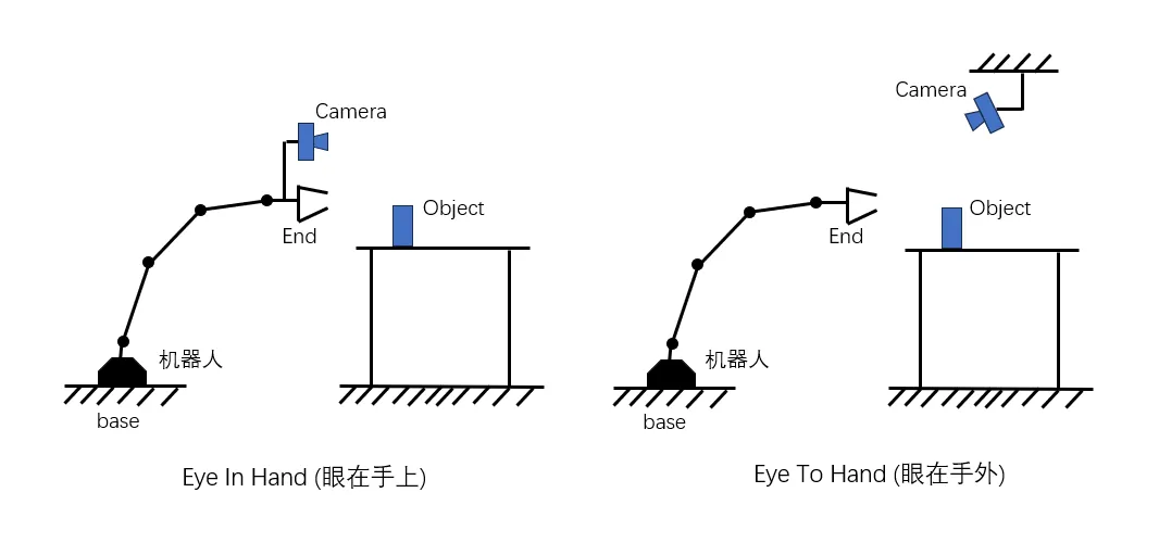
6.1.2 Mathematical Model of Hand-Eye Calibration
Whether the eyes are on the hand or outside the hand, the mathematical equation they solve is the same, which is
The relationships between coordinate systems are usually represented by the homogeneous transformation matrix (rigid body transformation) T:
mathT^i_j = \begin{bmatrix} R^i_j & t^i_j \\ 0 & 1 \end{bmatrix}
Among them, R ∈ SO(3) (rotation matrix, special orthogonal group) and t ∈ R³ (3D translation vector) correspond to rotation transformation and translation transformation respectively. The subscripts of T indicate which two coordinate systems the transformation applies to, for example:
6.1.2.1 Eye In Hand
When the camera is fixed at the end of the robotic arm, the transformation between the camera and the end effector remains constant. This is referred to as “eyes on the hand.” During such hand-eye calibration, a calibration plate is fixed in one location, and then the robotic arm is controlled to move to different positions. The camera mounted on the robotic arm takes photos of the calibration plate at various positions, resulting in multiple sets of images of the calibration plate at different locations.
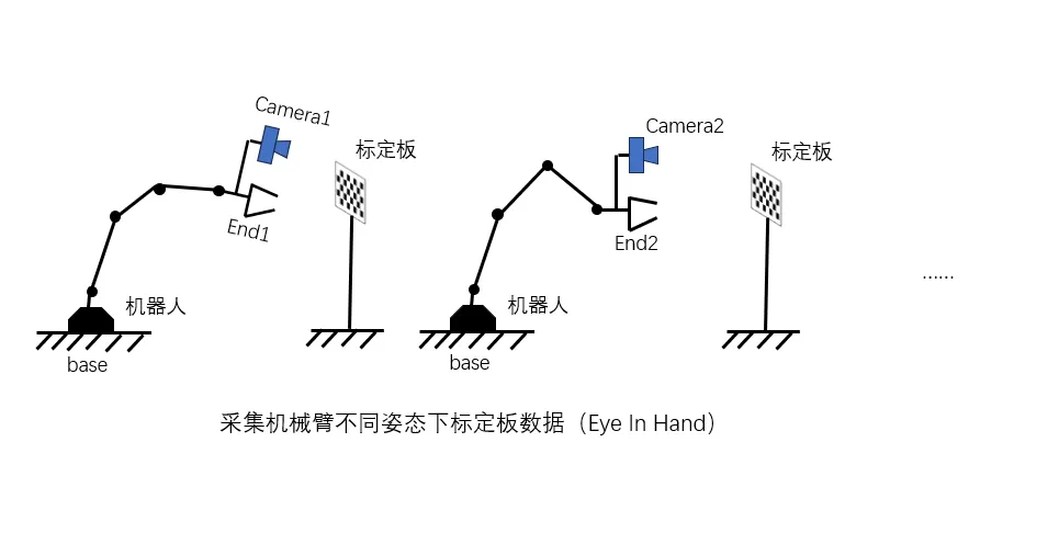
Since the calibration plate and the robot base are fixed, the relative pose relationship between them remains unchanged, thus:
mathT^b_t = T^b_{e1}\ T^{e1}_{c1}\ T^{c1}_{t} = T^b_{e2}\ T^{e2}_{c2}\ T^{c2}_{t}
Transform the above equation
math(T^b_{e2})^{-1}T^b_{e1}T^{e1}_{c1}T^{c1}_{t} = T^{e2}_{c2}T^{c2}_{t}
math(T^b_{e2})^{-1}T^b_{e1}T^{e1}_{c1} = T^{e2}_{c2}T^{c2}_{t}(T^{c1}_{t})^{-1}
mathT^{e2}_{e1}T^{e1}_{c1} = T^{e2}_{c2}T^{c2}_{c1}
mathT^{e2}_{e1}T^{e}_{c} = T^{e}_{c}T^{c2}_{c1}
mathAH = HB
Among them, T^e_c is the H that needs to be solved ultimately.
6.1.2.2 Eye To Hand
When the camera is positioned outside the robotic arm, the relative position between the camera and the end effector changes as the robotic arm moves. This condition is referred to as the eye outside the hand. For such hand-eye calibration, a calibration plate is fixed at the end of the robotic arm, and then the robotic arm is controlled to hold the calibration plate while taking photos around the fixed camera. To ensure accuracy in the solution, more than 10 sets of images are typically required.
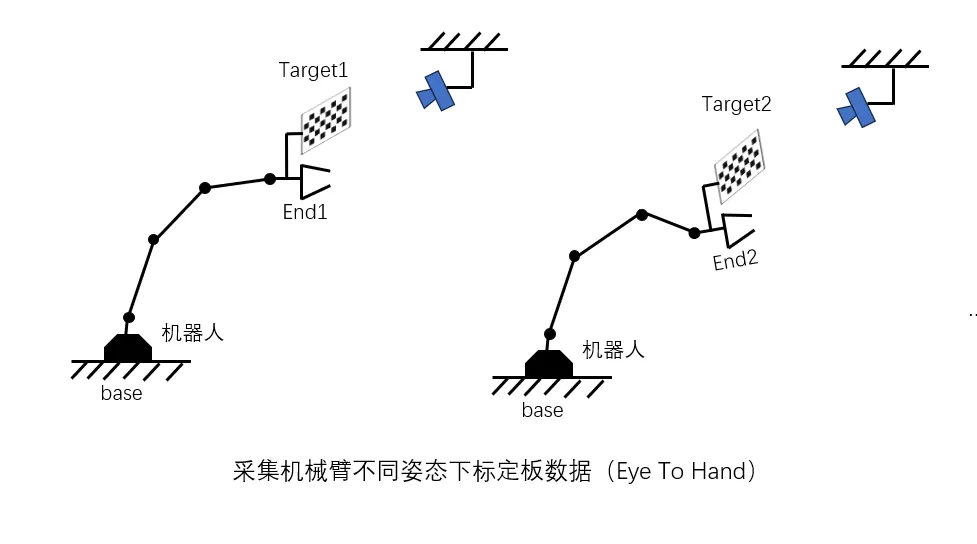
Since the calibration plate is fixed at the end of the robotic arm at this time, its relative position remains constant when taking different photos, thus:
mathT^e_t = T^{e1}_bT^{b}_{c}T^{c}_{t1} = T^{e2}_bT^{b}_{c}T^{c}_{t2}
Transform the above equation:
mathT^{e1}_bT^{b}_{c}T^{c}_{t1} = T^{e2}_bT^{b}_{c}T^{c}_{t2}
math(T^{e2}_b)^{-1}T^{e1}_bT^{b}_{c}T^{c}_{t1} = T^{b}_{c}T^{c}_{t2}
math(T^{e2}_b)^{-1}T^{e1}_bT^{b}_{c} = T^{b}_{c}T^{c}_{t2}(T^{c}_{t1})^{-1}
math(T^b_{e2}T^{e1}_b)T^{b}_{c} = T^{b}_{c}(T^{c}_{t2}T^{t1}_c)
mathAH = HB
6.1.3 Solving AH = HB
As an important aspect of robotics, the academic community has conducted extensive research on eye-hand calibration since the 1980s. Many AH = HB solving methods have been developed. Currently, the step-by-step method is commonly used. This method involves decomposing the system of equations and then utilizing the properties of rotation matrices to first solve for the rotation, and subsequently substituting the solution for the rotation into the translation solution to obtain the translation part.
Common two-step classic algorithms include the Tsai-Lenz method that converts the rotation matrix into a rotation vector, and the Park method that uses the properties of the rotation matrix in the Lie group (the adjoint property of the Lie group) for solution. Next, we will introduce the Park method.
6.1.3.1 Park method to solve the rotated
The three variables in the original equation are all homogeneous transformation matrices (homogeneous transformation: writing rotation and translation into a 4x4 matrix), representing the transformation between two coordinate systems. Its basic structure is as follows:
mathH = \left[\begin{array}{cc} R & t \\ 0 & 1 \end{array}\right]
Among them, R ∈ SO(3) (rotation matrix, special orthogonal group) and t ∈ R³ (3D translation vector) correspond to rotation transformation and translation transformation respectively.
Transform the original equation:
Therefore, (the product result rotates and translates such that the corresponding positions are equal):
First, solve the first equation that only contains a rotation matrix.
The rotation matrix belongs to the SO3 group, which is a Lie group. Each Lie group has a corresponding Lie algebra, which exists in a low-dimensional Euclidean space (linear space). It is represented as the tangent space of the local open domain of the Lie group. The Lie group and Lie algebra can be converted into each other via the exponential and logarithmic mappings:
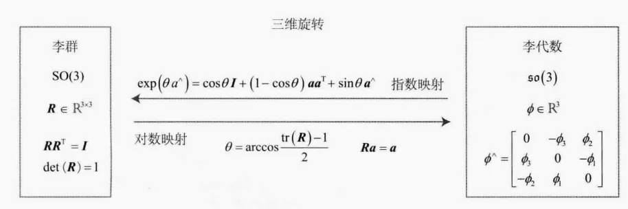 For the rotation matrix R, the transformation relationship with the corresponding Lie algebra
Φ can be expressed as follows:
The [ ] symbol indicates the ^ manipulation, which converts it into a antisymmetric matrix, or the cross product.
For SO(3), its adjoint property is:

When multiple sets of observations exist, the above problem can be transformed into the following least squares problem:

α and β are the Lie algebras corresponding to rotation, and both are three-dimensional vectors. They can be regarded as a three-dimensional point. Thus, the above problem is equivalent to a point cloud alignment problem:
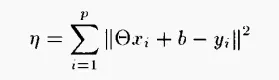
The least squares solution for this problem is:
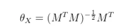
Among them:
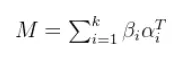
6.1.3.2 Park method for solving translation
After obtaining the rotation matrix through solving, substitute the rotation matrix into the second equation:
Here, C and D are known values. Since C is not necessarily invertible, the original equation is transformed as follows:
math\begin{aligned}
Cb_{X} &= D \\
C^TCb_{X} &= C^TD \\
b_{X} &= (C^TC)^{-1}C^TD
\end{aligned}
The translated part can be obtained.
When there are multiple sets of observation values

The final solution is:
math\begin{aligned}
H = \left[\begin{array}{cc}
\theta_{X} & b_{X} \\
0 & 1
\end{array}\right]
\end{aligned}
6.1.4 Hand-eye Calibration Methods in OpenCV and Calibration Precautions
According to the implementation principle, hand-eye calibration algorithms can be divided into three categories: independent closed solutions, simultaneous closed solutions, and iterative methods.
a. Independent closed-form solutions (seperable closed-form solutions): Solve the rotation component separately from the displacement components.
Disadvantage: The calculation error of the rotation component Rx will be carried into the calculation of the displacement component tx.
b. Simultaneous closed-form solutions (simultaneous closed-form solutions): Solve both the displacement component and the rotation component simultaneously.
Disadvantage: Due to noise, the solution of the rotation component Rx may not be a orthogonal matrix. Therefore, an orthogonalization step must be performed on the rotation component. However, the corresponding displacement components are not recalculated, which leads to solving errors.
c. Iterative solutions (iterative solutions): Use optimization techniques to iteratively solve the rotation component and the displacement component.
Disadvantage: This method may involve a large amount of computation, as it usually includes complex optimization procedures. Additionally, as the number of equations (n) increases, the difference between the iterative solution and the closed-form solution typically decreases. Thus, before using this method, it is necessary to determine whether the accuracy of the iterative solution is worth the computational cost.
6.1.4.1 Hand-eye Calibration Interface in OpenCV
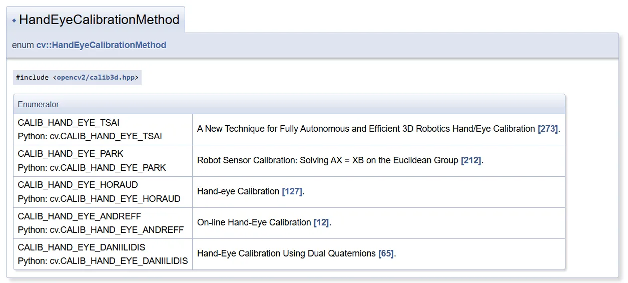
OpenCV mainly implements the first two types of methods, with the default method being TSAI. PARK and HORAUD also use independent solution methods. ANDREFF and DANIILIDIS provide closed-form solutions. (These results were obtained from the same dataset experiments; it is believed that the error in the solutions obtained by the TSAI method among independent solutions is relatively large.)
Collect multiple sets of calibration data, input it along with the robotic arm data and the camera calibration plate positioning data, and the calibration results can be obtained.
6.1.4.2 Calibration Precautions
When a beginner performs the first calibration, the following points need attention:
1: Using calibrateCamera to obtain the R and t matrices from the calibration plate to the camera, which is different from the internal parameters used for grasping, leads to errors.
- The direction of the corner point of the calibration plate is reversed. By default, it is from left to right, but sometimes it becomes from right to left, resulting in a non-unified coordinate system.
3: The calibration plate is too small, and it only moves in the center. This results in inaccurate edges.
4: Rotate during calibration
5: Too few images. More than 10 are required.
- Some cameras have issues; pay attention to the rgbd transformation matrix.
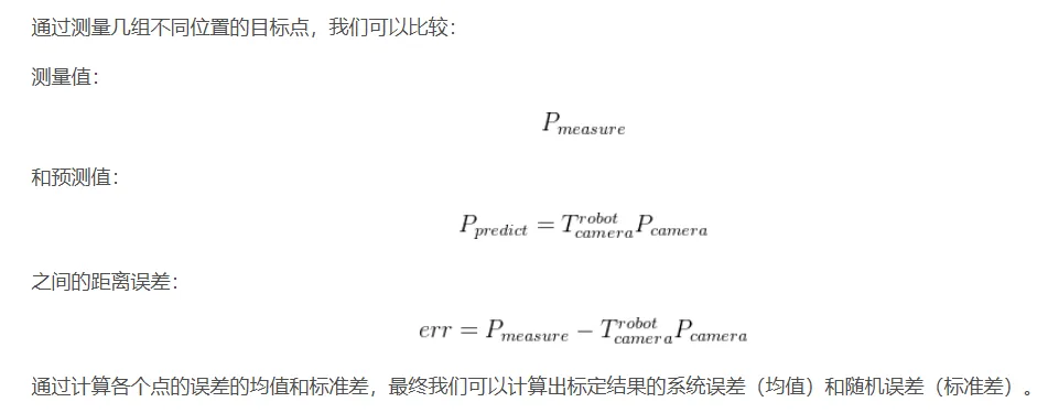
6.1.5 Evaluate the Hand-Eye Calibration Effect
References
2. Guide to Robot Hand-Eye Calibration
3. Calibration Learning Notes (4) – Detailed Explanation of Hand-Eye Calibration
4.Camera Calibration and 3D Reconstruction
5.3D Visual Workshop - Hand-Eye Calibration (with OpenCV implementation code)