1. Practical Exercise: UR5 Robot DH Parameter Table
UR5 is the most classic 6-degree-of-freedom collaborative robot in the industry. Below are its standard DH parameters (Note: Different manufacturers or literature may use improved DH, i.e., MDH. Here, standard DH is shown to comply with the definition in Document 2).
Unit:
| Joint (i) | αi (Twist) | ai (Link Length) | di (Link Offset) | θi (Range) |
|---|---|---|---|---|
| 1 (Base) | 0 | 89.16 | ||
| 2 (Shoulder) | 0 | -425.00 | 0 | |
| 3 (Elbow) | 0 | -392.25 | 0 | |
| 4 (Wrist 1) | 0 | 109.15 | ||
| 5 (Wrist 2) | 0 | 94.65 | ||
| 6 (Wrist 3) | 0 | 0 | 82.30 |
Practice exercise: Try to use the
forward_kinematicscode provided in Document 2, enter the above parameters, and calculate the end coordinate of UR5 when it is at zero position ().
2. Dynamics Simulation: Phase Diagram and Time-Domain Response of a Simple Pendulum
In Document 3, we derived the dynamics equation of a simple pendulum. Now, we use the Python scientific computing library scipy to perform numerical integration on it, simulating real physical motion.
Differential equation form:
We convert the second-order differential equation
Let the state vector be
3. Python simulation code (scipy.integrate.odeint)
Pythonimport numpy as np
from scipy.integrate import odeint
import matplotlib.pyplot as plt

# 1. 定义系统动力学方程 (导数函数)
def pendulum_dynamics(y, t, g, L, m, b):
    """
    y: 状态向量 [theta, omega]
    t: 时间点
    g, L, m, b: 物理参数
    """
    theta, omega = y

    # 状态方程:
    # d(theta)/dt = omega
    # d(omega)/dt = -(g/L)sin(theta) - (b/(mL^2))omega
    dydt = [omega, -(g/L)*np.sin(theta) - (b/(m*L**2))*omega]

    return dydt

# 2. 设置参数
g = 9.81   # 重力加速度
L = 1.0    # 杆长
m = 1.0    # 质量
b = 0.5    # 阻尼系数 (空气阻力等)

# 3. 初始条件
theta_0 = np.radians(179) # 初始角度 (接近顶点,测试非线性)
omega_0 = 0.0             # 初始角速度
y0 = [theta_0, omega_0]

# 4. 时间跨度
t = np.linspace(0, 10, 200) # 模拟 10 秒

# 5. 解微分方程
# odeint 自动使用数值积分方法求解
solution = odeint(pendulum_dynamics, y0, t, args=(g, L, m, b))

# 6. 绘图结果
theta_traj = solution[:, 0]
omega_traj = solution[:, 1]

plt.figure(figsize=(10, 6))

# 子图 1: 角度随时间变化
plt.subplot(2, 1, 1)
plt.plot(t, theta_traj, 'b-', label='Theta (rad)')
plt.title('Pendulum Dynamics Simulation (Damped)')
plt.ylabel('Angle (rad)')
plt.grid(True)
plt.legend()

# 子图 2: 相图 (Phase Portrait) - 速度 vs 角度
plt.subplot(2, 1, 2)
plt.plot(theta_traj, omega_traj, 'r-')
plt.title('Phase Portrait (State Space)')
plt.xlabel('Angle (rad)')
plt.ylabel('Angular Velocity (rad/s)')
plt.grid(True)
plt.tight_layout()

print("仿真完成,请查看绘图窗口。")
# 实际运行时请确保环境支持 plt.show()
# plt.show()
4. Result Analysis
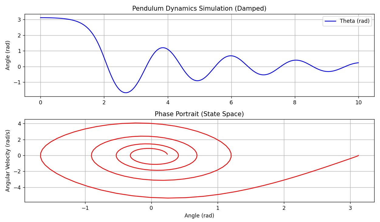
- Trajectory (upper figure): You will see a simple pendulum falling from a high position. After several oscillations, due to damping
, the amplitude gradually decreases and eventually approaches 0 (vertically downward). - Phase diagram (lower figure): It shows the trajectory of
and . It should be a spiral that contracts towards the origin, which intuitively demonstrates the system’s stability.