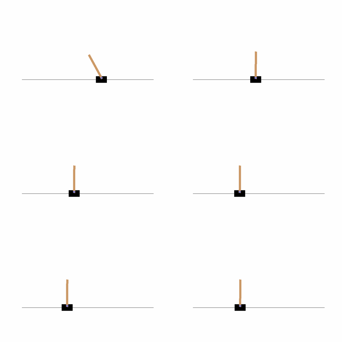
Python implementation of Cartpole modeling and PID, LQR, MPC control algorithms
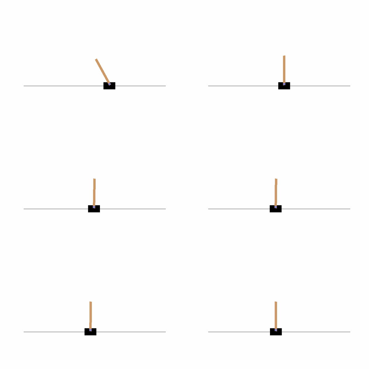
The goal of the CartPole problem is to keep the pole vertical (angle = 0) and the cart at the center of the track (position = 0).
The tutorial does not cover formula derivations. If you want to understand the underlying principles of PID\LQR\MPC, you can study it on your own.
I. Environment and Basics Used
- Windows
- Matrix Theory and Control Theory
- For environment installation, see requirments.txt
II. Cartpole Modeling
The code for the definition of the Cartploe official dynamics model is as follows: refer to http://incompleteideas.net/sutton/book/code/pole.c
For details, refer to the cartpole_env.py file in the code. During the implementation, in order to adapt to the linear controller, we made an approximation to the dynamics model, which will be introduced later.
python# temp = (force + self.polemass_length * theta_dot * theta_dot * sintheta) / self.total_mass
# thetaacc = (self.gravity * sintheta - costheta * temp) / (self.length * (4.0 / 3.0 - self.masspole * costheta * costheta / self.total_mass))
# xacc = temp - self.polemass_length * thetaacc * costheta / self.total_mass
The conversion into a formula can be expressed as:
For the linear controller, since the angle of the inverted pendulum
By organizing the above equation into a state space equation, we get:
The state space equations are used in LQR and MPC code. The corresponding Python code is as follows:
pythonA = np.eye(4) + del_t * np.array([[0, 1, 0, 0],
                [0, 0, (-3*m*g)/(m+4*M), 0],
                [0, 0, 0, 1],
                [0, 0, (3*(M+m)*g)/(L*(m+4*M)), 0]])
B = del_t * np.array([[0],
                [(1/(M+m))+((3*m)/(m+4*M))],
                [0],
                [-(3)/(L*(m+4*M))]])
III. Code Explanation
1. PID Controller
In the code, only PD control is used. Specifically, the deviation between the position of cart and the angle of pole is calculated, and then PD control is applied. The core code for PD control is as follows:
pythondef pid_cart(self, position):
    bias = position
    d_bias = bias - self.bias_cart_1
    balance = self.kp_cart * bias + self.kd_cart * d_bias
    self.bias_cart_1 = bias
    return balance

def pid_pole(self, angle):
    bias = angle  #
    d_bias = bias - self.bias_pole_1
    balance = -self.kp_pole * bias - self.kd_pole * d_bias
    self.bias_pole_1 = bias
    return balance
2. LQR controller
Discrete LQR Controller Problem Description:
The calculation steps for the discrete LQR controller are:
- Solve for the S matrix:
- Calculate the feedback matrix K:
- Calculate the control input u:
During the actual use of Cartpole in the LQR controller,
The core code of the LQR controller is as follows:
pythondef control_output(self, state_des, state_now):
    S = np.matrix(linalg.solve_discrete_are(self.A, self.B, self.Q, self.R))
    K = np.matrix(linalg.inv(self.B.T * S * self.B + self.R) * (self.B.T * S * self.A))
    # print("state_now", state_now)
    # print("state_des", state_des)
    action_list  = -10*np.dot(K, state_now - state_des)
    action = action_list[0,0]
    return action
The Lirakhtia equation is calculated using the solve_discrete_are function from the linalg library.
3. MPC Controller
Core components of MPC:
-
Prediction model: Used to predict the future state trajectory of the system based on the current state and future control inputs.
-
Scroll optimization: Find a set of control inputs that make the defined performance metric (cost function) optimal within the prediction horizon.
-
Feedback correction: Adjust the model prediction based on measurements, and re-predict and optimize at the next time point according to the new state.
Description of the linear MPC problem:
Among them:
is the prediction step size (prediction interval). is the prediction of the state at at the moment . is the control input scheduled at at the moment . is the state weight matrix. is the control input weight matrix. is the terminal state weight matrix.
The core code of the MPC controller is as follows:
- Construct the matrix for the QP problem: The purpose is to calculate the matrices H and E in the QP formula.
pythondef get_QPMatrix(A, B, Q, R, F, N):
    M = np.vstack([np.eye(n), np.zeros((N*n, n))])
    C = np.zeros(((N+1)*n, N*p))
    temp = np.eye(n)
    for i in range(1,N+1):
        rows = i * n + np.arange(n)
        C[rows,:] = np.hstack([temp @ B, C[rows-n, :-p]])
        temp = A @ temp
        M[rows,:] = temp

    Q_ = np.kron(np.eye(N), Q)
    rows_Q, cols_Q = Q_.shape
    rows_F, cols_F = F.shape
    Q_bar = np.zeros((rows_Q+rows_F, cols_Q+cols_F))
    Q_bar[:rows_Q, :cols_Q] = Q_
    Q_bar[rows_Q:, cols_Q:] = F
    R_bar = np.kron(np.eye(N), R)

    # G = M.T @ Q_bar @ M
    E = C.T @ Q_bar @ M
    H = C.T @ Q_bar @ C + R_bar
    return E, H
- Online MPC solution
CasADi: This is a powerful symbolic computation and automatic differentiation framework, commonly used to solve optimal control and nonlinear optimization problems.
pythondef mpc_prediction(x_k, E, H, N, p):
    # 定义优化变量
    U = ca.SX.sym('U', N * p)
    # 定义目标函数
    objective = 0.5 * ca.mtimes([U.T, H, U]) + ca.mtimes([U.T, E, x_k])
    qp = {'x': U, 'f': objective}
    opts = {'print_time': False, 'ipopt': {'print_level': 0}}
    solver = ca.nlpsol('solver', 'ipopt', qp, opts)

    # 求解问题
    sol = solver()
    # 提取最优解
    U_k = sol['x'].full().flatten()
    u_k = 10*U_k[:p]  # 取第一个结果

    return u_k
IV. Code Results
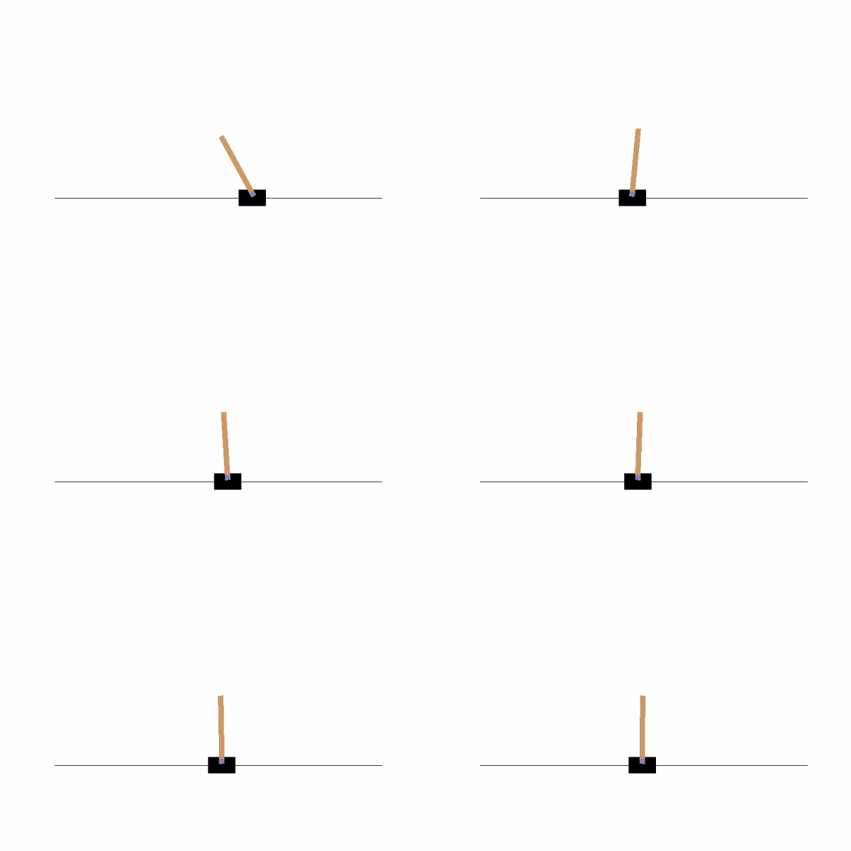
1. PID Control Results
2. LQR Control Results
3. MPC Control Results