Detailed Explanation of VAE and Implementation of MNIST Image Generation

This tutorial provides a comprehensive explanation from the motivation behind VAE, probability models, ELBO derivation, and final training objectives, to the code implementation for generating MNIST images. The focus is on understanding why VAE is designed in this way, and how to determine whether the model has truly learned a usable latent space during training and generation.

0. Learning Path

The main process of VAE can be compressed into four steps:

1. Ordinary Autoencoder can reconstruct, but the latent space may not allow random sampling.
2. The latent variable generation model can describe “first sampling $z$, then generating $x$”, but the edge likelihood $\log p_{\theta}(x)$ is difficult to compute directly.
3. VAE introduces an approximate posterior $q_{\phi}(z|x)$, using ELBO instead of the real likelihood which cannot be directly optimized.
4. The training objective ultimately becomes “reconstruction loss + KL loss”, requiring both good reconstruction and a latent space close to a standard normal distribution.

VAE is a generative model with a probabilistic latent space. It combines the reconstruction capability of Autoencoder and the probabilistic modeling of variational inference, enabling the model to sample from a simple prior $p(z)=\mathcal{N}(0,I)$ and generate new data.

1. Why VAE is needed

1.1 What the generation model really wants to learn

Given training data:

The generation model aims to learn the real data distribution:

Here, $x$ represents data, and $\theta$ represents model parameters. The maximum likelihood training objective is:

This target indicates that real samples should have a high probability under the model distribution.

After being trained, the generative model should be able to:

• Determine whether a sample resembles real data;
• Randomly sample new samples from the model;
• Interpolate and control in the latent space;
• Learn the low-dimensional structure behind the data.

1.2 Problems of Ordinary Autoencoders

The structure of a standard Autoencoder is:

Its goal is to make the reconstruction result $\hat{x}$ close to the original input $x$:

Ordinary AE is suitable for compression, dimensionality reduction, noise removal, and feature learning, but it is not inherently a generative model. This is because the Encoder output of a ordinary AE is a fixed point:

This only ensures that the training samples can be mapped near certain latent variable points, but does not guarantee that the entire latent space is continuous, regular, and sampleable.

Therefore, three problems will arise:

1. There may be voids in the潜 space.
2. Randomly sampled $z$ may not generate reasonable samples.
3. When performing插 value on潜 variables between two samples, the middle region may be meaningless.

The regular AE can be reconstructed, but its generation is not guaranteed.

1.3 Natural Idea of Hidden Variable Generation Models

To generate data, it can be assumed that there is a latent variable behind each sample $z$. The generation process is as follows:

Common prior is a standard normal distribution:

The joint distribution is:

If this model can be trained, during generation, we only need to sample from $p(z)$ first, and then use the Decoder to generate $x$.

1.4 Why Direct Training of Hidden Variable Models Is Difficult

In the training data, there is only $x$, and no corresponding $z$. Therefore, the training objective requires edge likelihood:

If the Decoder is a neural network, this integral is usually unsolvable. Reasons include:

• $z$ is a high-dimensional continuous variable;
• $p_{\theta}(x|z)$ is defined by a complex nonlinear neural network;
• There is no analytical solution for the integration;
• Performing numerical integration for each sample is extremely costly.

The true a-posteriori cannot be directly calculated:

Since the denominator $p_{\theta}(x)$ is unsolvable, $p_{\theta}(z|x)$ is also unsolvable.

The key creativity of VAE lies here: using a trainable approximate posterior $q_{\phi}(z|x)$ instead of the true posterior $p_{\theta}(z|x)$, and then constructing an optimizable lower bound.

1.5 Basic Model of VAE

VAE contains three probability objects:

1. Prior distribution:

2. Generate distribution:

3. Approximate posterior:

In neural network implementation:

• Encoder refers to $q_{\phi}(z|x)$;
• Decoder refers to $p_{\theta}(x|z)$;
• Standard normal distribution refers to $p(z)$.

The Encoder no longer outputs a single latent variable point, but instead outputs a distribution:

That is, output the mean $\mu$ and the log variance $\log\sigma^2$. Then sample from this distribution using $z$, and send it to the Decoder for reconstruction or generation.

The core difference between VAE and ordinary AE is:

This change transforms the latent variable from “a coding point” into “a probability distribution”, thus providing a foundation for random generation and the regularization of the latent space.

2. Model derivation of VAE

This chapter only discusses two derivation paths. They yield the same ELBO, but the questions they answer are different.

• Route 1: Jensen’s Inequality Approach Answer the question: “Why can an unsolvable $\log p_{\theta}(x)$ be turned into a feasible lower bound?”

• Route 2: Likelihood Decomposition Route Answering “What exactly is the difference between ELBO and the real $\log p_{\theta}(x)$?”.

2.1 Route 1: Deriving a Trainable Lower Bound from Jensen’s Inequality

The goal of this route is to start from the training objectives and construct an optimal lower bound that can be optimized.

VAE originally wanted to maximize the edge log likelihood:

The problem here is that the integrals are unsolvable. Since there is only $x$ in the training data, and the latent variable $z$ is not observable, all possible $z$ must be integrated.

Step 1: Multiply or divide by a distribution $q_{\phi}(z|x)$ in the integration:

This step does not change the values, as it is simply multiplying and dividing by the same quantity simultaneously. The purpose of this is to rewrite the integral as an expectation regarding $q_{\phi}(z|x)$:

Step 2: Use Jensen’s inequality to substitute $\log$ into the expectation. Since $\log$ is a concave function:

Let:

Result:

On the right is ELBO:

Therefore, VAE does not directly optimize the unsolvable $\log p_{\theta}(x)$, but optimizes its lower bound:

Next, expand ELBO into an achievable loss. From the joint distribution:

Available:

Separate the reconstruction items and KL items:

This is the conclusion of Route 1:

It has two parts:

• $\mathbb{E}_{q_{\phi}(z|x)}[\log p_{\theta}(x|z)]$: Reconstruction item, encouraging the Decoder to restore $x$ from $z$;
• $D_{KL}(q_{\phi}(z|x)\|p(z))$: A prior constraint, encouraging the Encoder’s output distribution to be close to a standard normal distribution.

During training, the negative ELBO is usually minimized:

That is:

If:

And:

Then the KL term has an analytical solution:

If the network output is $\log\sigma^2$, denoted as logvar, is usually written as:

2.2 Route 2: Understanding the Gap Between ELBO and Likelihood Decomposition

This approach does not use the Jensen inequality initially, but instead splits the true log-likelihood into two parts. Its goal is to explain why ELBO represents a lower bound, and how far this lower bound is from the true objective.

Because $\log p_{\theta}(x)$ has nothing to do with $z$:

Next, rewrite $p_{\theta}(x)$ using a Bayesian relationship. By:

Available:

Then introduce $q_{\phi}(z|x)$ into the fraction:

Break down the multiplication in the logarithm into addition:

The first item is ELBO:

The second item is the KL divergence between the approximate posterior and the true posterior:

So, the result is:

Because the KL divergence is always non-negative:

So:

This is the conclusion of Route 2:

ELBO is the lower bound because there is a non-negative posterior KL difference between it and the real $\log p_{\theta}(x)$.

This route also explains the different roles of two KLs:

• $D_{KL}(q_{\phi}(z|x)\|p_{\theta}(z|x))$: The theoretical posterior gap, used to explain the difference between ELBO and the true likelihood, but cannot be directly trained due to the intractable true posterior;
• $D_{KL}(q_{\phi}(z|x)\|p(z))$: The prior constraint in the training loss, which can be calculated directly to make the latent space close to a standard normal distribution.

The two routes achieve the same training objective. The final VAE model is:

• The encoder outputs $\mu$ and $\log\sigma^2$;
• $z$ is obtained through reparameterization;
• The decoder reconstructs or generates images from $z$;
• The loss consists of reconstruction loss and KL loss.

3. VAE Code Implementation

This section explains the implementation method with code snippets. The complete code is located at:

• code/train_mnist_unet_vae.py
• code/generate_mnist_unet_vae.py

The dataset uses the mnist dataset and will be downloaded automatically. There is no need to worry about issues with the dataset; you only need to install torch properly.

The model here uses a U-Net-style convolutional downsampling and upsampling structure. Note that during the generation phase, there are only random latent variables $z$, and no input images exist, so it cannot rely on cross-layer skip features of the input images. The code adopts a “U-Net-style hierarchical convolutional structure” instead of relying on the full U-Net of the input skip features.

3.1 Model Structure

The core model in the training script is UNetVAE. The Encoder downsamples the MNIST images of $1\times28\times28$ to high-dimensional features, and then outputs mu and logvar:

pythonself.enc1 = nn.Sequential(nn.Conv2d(1, base, 3, padding=1), nn.GroupNorm(4, base), nn.SiLU())
self.enc2 = nn.Sequential(nn.Conv2d(base, base * 2, 4, stride=2, padding=1), nn.GroupNorm(8, base * 2), nn.SiLU())
self.enc3 = nn.Sequential(nn.Conv2d(base * 2, base * 4, 4, stride=2, padding=1), nn.GroupNorm(8, base * 4), nn.SiLU())
self.fc_mu = nn.Linear(base * 4 * 7 * 7, latent_dim)
self.fc_logvar = nn.Linear(base * 4 * 7 * 7, latent_dim)

The Decoder projects the latent variable $z$ back to the $7\times7$ feature map, and then gradually upsamples it back to $28\times28$:

pythonself.fc_dec = nn.Linear(latent_dim, base * 4 * 7 * 7)
self.dec1 = nn.Sequential(nn.ConvTranspose2d(base * 4, base * 2, 4, stride=2, padding=1), nn.GroupNorm(8, base * 2), nn.SiLU())
self.dec2 = nn.Sequential(nn.ConvTranspose2d(base * 2, base, 4, stride=2, padding=1), nn.GroupNorm(4, base), nn.SiLU())
self.out = nn.Conv2d(base, 1, 3, padding=1)

The output layer does not directly connect to sigmoid, and binary_cross_entropy_with_logits is used during training. This makes the values more stable.

3.2 Reparameterization

The original sampling format is:

Reparameterized as:

Code snippet is:

pythonstd = torch.exp(0.5 * logvar)
eps = torch.randn_like(std)
z = mu + std * eps

This randomness comes from eps, while z is a differentiable function of mu and logvar. The gradient can be transmitted back from the Decoder to the Encoder.

After reparameterization, what is actually calculated during model training is a differentiable estimate of the negative ELBO. For a training sample $x$, the calculation process can be written as:

Therefore, the training objective for a single sample is:

If the output distribution of the Decoder is set to a Gaussian distribution:

After ignoring constants unrelated to model parameters, the reconstruction term is equivalent to the mean square error. The formula for true optimization can be written as:

The first item here is the reconstruction error, and the second item is the KL divergence between $q_{\phi}(z|x)$ and the standard normal prior $p(z)=\mathcal{N}(0,I)$. When actually training a mini-batch, the samples within the batch are usually averaged:

In the following MNIST code, the Encoder output is logvar, which is $\log\sigma^2$. Therefore, the KL term is written as:

If the reconstruction item uses binary_cross_entropy_with_logits, then the total loss in the code is the achievement of this batch goal:

3.3 Training Objectives

The MNIST pixels are normalized to $[0,1]$, so the reconstruction term uses binary cross-entropy. The logits version is used in the training script:

pythonrecon_loss = F.binary_cross_entropy_with_logits(recon_logits, x, reduction="sum") / x.size(0)
kl_loss = -0.5 * torch.sum(1 + logvar - mu.pow(2) - logvar.exp()) / x.size(0)
loss = recon_loss + beta * kl_loss

Here, beta is the KL weight. You can use KL warm-up in the early stage of training:

pythonbeta = min(1.0, epoch / max(1, args.warmup_epochs)) * args.beta

In this way, the model first learns basic reconstruction, and then gradually strengthens the latent space constraints, which can alleviate the disappearance of KL.

3.4 Output of Training Script

train_mnist_unet_vae.py will be saved:

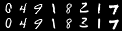
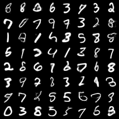
• checkpoints/mnist_unet_vae.pt: Model weights and configuration;
• outputs/recon_epoch_XXX.png: Comparison between the original image and the reconstructed image;
• outputs/sample_epoch_XXX.png: Images generated from standard normal prior sampling.

Operation mode:

bashpython train_mnist_unet_vae.py --epochs 20 --batch-size 128 --latent-dim 32

If the machine has CUDA, the script will automatically use the GPU.

The execution result is as follows:

(1) Result of original image reconstruction

(2) Sampling Generation Results

3.5 Test Generation Script

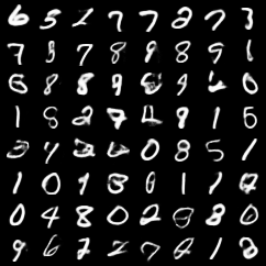
generate_mnist_unet_vae.py is used only for generation:

1. Load the trained checkpoint;
2. Sample from $z\sim\mathcal{N}(0,I)$;
3. Pass it to the Decoder;
4. Save the generated image grid.

Operation mode:

bashpython generate_mnist_unet_vae.py --checkpoint checkpoints/mnist_unet_vae.pt --num-samples 64

The generation script does not require training data; it relies solely on the trained Decoder.

The test generation results are as follows:

3.6 Implementation Tips

1. Prioritize outputting logvar Direct output of variance may result in negative values or numerical explosions. Outputting log variance is more stable.

2. Reconstruction loss and KL loss should be recorded separately It is not sufficient to only look at the total loss. When KL is close to 0, it may indicate that latent variables are not being used.

3. Save the mapping and sampling image The mapping shows whether the Encoder-Decoder can compress and restore; the sampling image indicates whether the latent space can generate results.

4. The U-Net-style structure should be adapted to the generation task The cross-layer skip connection of traditional U-Net relies on the input image. Since there is no input image during VAE generation, this implementation uses a hierarchical convolutional structure and does not use skip concatenation that depends on the input.

5. Do not blindly increase the latent variable dimensions For MNIST, you can start with 16, 32, or 64. If the dimension is too small, the reconstruction will be poor; if it is too large, some dimensions may remain unused.

4. Common Issues

5.1 Is VAE just an ordinary AE with noise?

No. The core of VAE is the probabilistic latent variable model and the ELBO training objective. Noise is just a part of the sampling from the posterior distribution.

5.2 Why VAE can generate images from random $z$

During training, the KL term brings $q_{\phi}(z|x)$ close to $p(z)=\mathcal{N}(0,I)$. Therefore, after training, $z$, sampled from a standard normal distribution, is more likely to fall in the region familiar to the Decoder.

5.3 Why use logits in training code

When using binary cross-entropy for MNIST, binary_cross_entropy_with_logits is more stable than sigmoid followed by BCE. sigmoid is applied to the logits when generating and saving images.

5.4 Why Not Use the Traditional U-Net Input Skip

The skip connection in the traditional U-Net extracts features from the input image and passes them to the Decoder. During the VAE generation phase, there is no input image, only random $z$s, so this input feature cannot be relied upon. Here, a U-Net-style convolution downsampling and upsampling structure is used.

5. Summary

The final VAE model consists of three parts:

The final training objective is:

Among them:

The value of VAE lies in the fact that it not only allows the model to reconstruct inputs, but also organizes data into a continuous, regular, and sampleable latent space. This latent space makes random generation, interpolation, and representation learning possible.

6. After-class Exercises

1. Why cannot a regular AE ensure valid random sampling?
2. Why does VAE have the Encoder output a distribution rather than a point?
3. Why is $\log p_{\theta}(x)$ difficult to optimize directly?
4. How is ELBO derived from Jensen’s inequality?
5. What does $\log p_{\theta}(x)=ELBO+KL(q_{\phi}(z|x)\|p_{\theta}(z|x))$ indicate?
6. Why is the KL term in the training loss $KL(q_{\phi}(z|x)\|p(z))$?
7. Why can the reparameterization trick make the sampling process trainable?
8. What might it mean when the KL loss approaches 0?
9. Why should we consider both the reconstruction image and random sampling image when evaluating VAEs?