Detailed Explanation and Code Implementation of DDPM

This tutorial starts from the limitations of VAE, explains why DDPM changes “single-step generation” to “multi-step denoising”, and then derives from forward diffusion, reverse generation, ELBO, true posterior, and noise prediction objectives to the final training and sampling formulas.

0. Learning Path

The main process of DDPM can be compressed into five steps:

1. VAE generates images in one step using latent variables $z$, but the assumptions of compression and reconstruction often lead to detail loss.
2. DDPM does not immediately generate a complete image; instead, it defines a fixed noise addition process to gradually transform the real image into Gaussian noise.
3. During generation, it starts from Gaussian noise, and the neural network is trained to remove a little bit of noise at each step.
4. The derivation strictly comes from maximum likelihood and ELBO, but it can ultimately be simplified into a straightforward supervision task: predicting the noise added to the image.
5. The key to implementation is not the complex loss function, but properly handling the noise schedule, time steps, U-Net input/output, sampling formulas, and numerical ranges.

DDPM first gradually adds noise to the image until it is close to pure noise, and then trains the model to gradually remove the noise in reverse. It breaks the difficult “one-step image generation” process into many simple “predict and remove noise” tasks.

The most common training objective for DDPM is:

Among them:

In other words, during training, we know the true noise $\epsilon$, and the network only needs to predict it based on the noisy image $x_t$ and the time step $t$.

1. Why DDPM is needed

1.1 Several Issues with VAE

VAE is important, but it also has several common issues.

First, VAE typically compresses images into a low-dimensional latent variable:

If the capacity of $z$ is insufficient, details will be lost, and the generated image will be blurry.

Second, the reconstruction terms of VAE often correspond to pixel-level likelihoods. Taking Gaussian likelihood as an example, maximizing $\log p_\theta(x|z)$ is often equivalent to minimizing mean squared error. Mean squared error encourages the model to output a “average answer,” and an average image usually looks dull.

Third, VAE generates $x$ directly from $z$ in one step:

This requires the Decoder to generate from abstract semantics to all pixel details during a single forward propagation. For complex images, this mapping burden is quite high.

Therefore, the core contradiction of VAE can be understood as:

It wants to generate images using a structured, sampleable latent space, but this compression and one-step decoding process may lose high-frequency details.

1.2 How DDPM Changes Its Approach

DDPM no longer views generation as:

Instead, consider it as:

Among them:

• $x_0$ is a real and clean image;
• $x_1,\dots,x_T$ is an image with noise added gradually;
• $x_T$ is close to standard Gaussian noise.

Sample first during generation:

Then, for each step, only a small task is done:

Predict the noise based on the current noisy image, and remove a little bit of it.

The benefits of DDPM are:

1. The training objective is stable, eliminating the need for adversarial training like that of GANs.
2. Each task step is simple, requiring only local denoising learning.
3. Generation occurs gradually in the image space, without forcing all details into a very small latent variable.
4. U-Net can be used to preserve multi-scale spatial details.
5. Mathematically, it is possible to derive a simple noise prediction MSE from ELBO.

2. Basic Settings of DDPM

DDPM has two processes:

1. Forward diffusion process: Fixed rules, no learning required; gradually add noise to the real image.
2. Reverse generation process: Requires learning; gradually remove noise to generate the image.

2.1 Forward Diffusion Process

The forward process starts from the real image $x_0$:

DDPM defines it as a Markov chain:

A Markov chain means: if $x_{t-1}$ is already known, then when generating $x_t$, there is no need to directly refer to earlier states.

Each step of noise addition is defined as:

Here:

• $\beta_t$ is the noise intensity at step $t$;
• $\beta_t I$ indicates that the variance of independent Gaussian noise of $\beta_t$ is added to each dimension;
• $\sqrt{1-\beta_t}x_{t-1}$ means retaining a portion of the image signal from the previous moment.

General definition:

So:

2.2 Writing the sampling formula from distribution

If:

It can be written as:

Apply this rule to the one-step forward distribution of DDPM:

Obtained:

Among them:

This is the step-plus-noise formula.

2.3 Why the coefficient uses a square root

Many beginners ask: Why is it $\sqrt{1-\beta_t}$, rather than $1-\beta_t$?

Assume that the variance of $x_{t-1}$ is approximately $I$, and the variance of noise $\epsilon_t$ is also $I$. If:

Then the variance is approximately:

In other words, after adding noise to each step, the overall scale does not suddenly increase or decrease.

If changed to:

Then the variance will become:

It is no longer exactly equal to $I$. Therefore, DDPM uses a square root coefficient to maintain a stable ratio between the variance of the signal and the noise.

3. From one-step noise addition to noise addition at any time

When training DDPM, it is very slow to add noise step by step from $x_0$ to $x_t$ every time. Fortunately, the forward process has a closed-form formula, allowing us to directly obtain $x_t$ at any time step from $x_0$.

The final formula is:

Among them:

The corresponding sampling formula is:

Among them:

This formula is very important. It indicates that during training, a random time step $t$ can be selected, and then the corresponding noisy image $x_t$ can be constructed in one go.

3.1 Two-step expansion to understand closed-form formulas

One-step noise addition is:

Write down the previous moment again:

Substitute the first equation:

Expand:

The last two items are linear combinations of independent Gaussian noise, so they are still Gaussian noise. Its variance is:

Therefore, it can be merged into a new standard Gaussian noise $\epsilon$:

Continuing the recursion to $x_0$, we get:

Definition:

We get the formula at any given moment:

3.2 Why $x_T$ approaches standard Gaussian noise

Because:

And:

When $t$ is large enough:

Insert:

The first item will disappear:

The second item will become:

So:

This explains why generation can start from pure Gaussian noise.

4. Diffusion Process in Reverse

The forward process is artificially fixed and does not require learning. What actually needs to be learned is the reverse process:

The model joint distribution is written as:

Among them:

The reverse step is usually also set as a Gaussian distribution:

Here:

• $\mu_\theta(x_t,t)$ is the reverse mean predicted by the neural network;
• $\sigma_t^2I$ is the reverse variance, which is not learned in many basic implementations;
• The network input is the noisy image $x_t$ and the time step $t$;
• The network output can be designed to predict the mean, predict the original image $x_0$, or predict the noise $\epsilon$.

Intuitively, the reverse step is done as follows:

Given the current noise map $x_t$, guess where the slightly cleaner image $x_{t-1}$ from the previous step should be located.

5. Training objective: From maximum likelihood to ELBO

As a generative model, DDPM aims to maximize the likelihood of real images:

But:

This integration requires integrating all intermediate variables $x_1,\dots,x_T$, and direct calculation is difficult.

Therefore, DDPM uses the variational lower bound. Minimize the negative ELBO during training:

Among them:

Detailed algebraic derivations are provided in Appendix A. The main text only retains the conclusions:

It has three types of items.

Item 1:

It indicates that the final noise distribution should be close to standard Gaussian. When $T$ is large enough, $q(x_T|x_0)\approx\mathcal{N}(0,I)$, this term is usually close to a constant.

Intermediate item:

It is the core of training. It requires the model to learn a reverse step distribution $p_\theta(x_{t-1}|x_t)$ that is close to the true posterior $q(x_{t-1}|x_t,x_0)$.

Last item:

Indicates the reconstruction error of restoring $x_0$ from $x_1$.

So the key issue of DDPM becomes:

How to make a neural network approximate the true posterior $q(x_{t-1}|x_t,x_0)$?

6. Real posterior and mean matching

True a posteriori is:

It indicates: If the original image $x_0$ and the noisy current image $x_t$ are known, what distribution should the state at the previous moment $x_{t-1}$ have been?

According to the Bayes’ formula:

Since the forward process is a Markov chain:

So:

The three distributions on the right are all Gaussian, so the result is still Gaussian:

Among them:

And:

The detailed formula derivation is provided in Appendix B. First, understand its meaning in the main text:

• The true posterior mean $\tilde{\mu}_t(x_t,x_0)$ is a linear combination of $x_0$ and $x_t$;
• It tells us the most reasonable center position when taking a step back from $x_t$;
• During model training, the mean predicted by the model $\mu_\theta(x_t,t)$ can be adjusted to approach this true mean.

Model reverse distribution is:

If the fixed variance is maintained, then the part of the KL between the two Gaussian distributions that is related to the model is the mean MSE:

Here, $C$ is a constant independent of the model parameter $\theta$.

This step transforms the complex probability matching problem into:

Make the reverse mean predicted by the model close to the true posterior mean.

7. From Prediction Mean to Prediction Noise

Theoretically, the network can directly predict:

However, in DDPM practice, prediction noise is more common:

This step seems sudden, but it actually comes from rewriting the formula.

7.1 Start with predicting $x_0$

The true posterior mean can be written as:

Among them:

When generating, the real $x_0$ is unknown, so the original image can be predicted by the network:

Reconstruction:

This indicates that the predicted original image $x_0$ and the predicted mean $\mu_\theta$ can be converted into each other.

7.2 Change the prediction from $x_0$ to prediction noise

The forward noise addition formula is:

Solve it against $x_0$:

If the network prediction noise:

The original image can be reconstructed for prediction:

Substitute $x_{0,\theta}$ into $\mu_\theta$ from the previous section, to obtain the most common reverse mean parameterization for DDPM:

The complete algebraic simplification of this formula is provided in Appendix C.

7.3 Why Predictive Noise Is Preferred

There are three intuitive advantages of prediction noise.

First, the supervision signals are naturally available. We sample them during training:

Then construct:

So the real noise $\epsilon$ is a known label.

Second, the target format is consistent. No matter how complex the image content is, the noise always comes from standard Gaussian:

Third, the sampling formula is intuitive. The model predicts the noise in the current image, and then subtracts it from $x_t$.

8. Final Training Objectives and Sampling Formulas

8.1 From Mean Matching to Noise Prediction MSE

The true posterior mean can be written in a noisy form:

The model mean is written as:

Subtract the two:

Therefore:

By substituting the mean-matching term corresponding to KL, a weighted noise prediction MSE is obtained:

In DDPM practice, simplified objectives are often used, and complex weights are removed:

Among them:

This is the most common training objective for DDPM.

8.2 Training Process

One training iteration can be understood as:

1. Sample real images from the dataset:

2. Random sampling time steps:

3. Sampling Gaussian noise:

4. Construct noisy images:

5. Introduce network prediction noise:

6. Minimize noise prediction error:

8.3 Sampling Process

After training is completed, start from pure noise:

Then perform it step by step from $t=T$ to $t=1$:

Among them:

Insert the mean value in the noise prediction form:

Usually, no random noise is added in the last step $t=1$, that is:

This can prevent the final output from being further disturbed.

9. DDPM Code Implementation

This section explains how DDPM is implemented in PyTorch from the STL10 code. The complete code is available at:

• code/train_stl10_ddpm.py
• code/generate_stl10_ddpm.py

The dataset uses STL10. split="train" is used in the code, and the image is adjusted to $96\times96$ by default. The dataset will be automatically downloaded during the first run. torch and torchvision must be installed in advance.

This implementation uses the most basic DDPM configuration: a linear beta schedule, noise-prediction objective, MSE loss, and a small U-Net noise predictor. Its goal is not to generate the strongest diffusion model in one go, but to first achieve a closed loop where noise is added during training, the model predicts noise, and noise is gradually removed during sampling.

9.1 Dataset and Image Scope

STL10 is a RGB image, so the model input shape is:

In the training script, first resize the images to the specified size, and then normalize the pixels to $[-1,1]$:

pythontransform = transforms.Compose(
    [
        transforms.Resize((args.image_size, args.image_size)),
        transforms.ToTensor(),
        transforms.Normalize((0.5, 0.5, 0.5), (0.5, 0.5, 0.5)),
    ]
)
train_set = datasets.STL10(
    root=args.data_dir,
    split="train",
    download=True,
    transform=transform,
)

Here, the Normalize((0.5,0.5,0.5),(0.5,0.5,0.5)) will convert the original $[0,1]$ pixels into $[-1,1]$:

The reason for this is that DDPM gradually brings the image closer to standard Gaussian noise. When the image range approaches $[-1,1]$, the data scale and noise scale become more consistent. When saving the generated image, the result is mapped back to $[0,1]$:

pythonutils.save_image((images + 1) / 2, out_path, nrow=int(num_samples**0.5))

9.2 Time Embedding

The DDPM network cannot only consider the noisy image $x_t$, but also must know the current time step $t$. The same image has a completely different noise level in $t=50$ and $t=900$. Without time information, the network doesn’t know how much noise to remove.

In the code, sine time embedding is used to convert integer time steps into continuous vectors:

pythonclass SinusoidalTimeEmbedding(nn.Module):
    def __init__(self, dim: int) -> None:
        super().__init__()
        self.dim = dim

    def forward(self, t: torch.Tensor) -> torch.Tensor:
        half = self.dim // 2
        freq = torch.exp(
            -math.log(10000)
            * torch.arange(half, device=t.device, dtype=torch.float32)
            / max(half - 1, 1)
        )
        angles = t.float()[:, None] * freq[None, :]
        emb = torch.cat([angles.sin(), angles.cos()], dim=-1)
        return F.pad(emb, (0, self.dim % 2))

The obtained time vector is further processed through MLP:

pythonself.time_mlp = nn.Sequential(
    SinusoidalTimeEmbedding(time_dim),
    nn.Linear(time_dim, time_dim),
    nn.SiLU(),
    nn.Linear(time_dim, time_dim),
)

In this way, each time step has a condition vector available for the network to use.

9.3 How the residual block injects time information

Each residual block in U-Net receives two inputs: image features x and temporal features time_emb. The temporal features are first projected through a linear layer to the current number of channels, and then added to the convolutional feature map:

pythonclass ResBlock(nn.Module):
    def __init__(self, in_ch: int, out_ch: int, time_dim: int) -> None:
        super().__init__()
        self.conv1 = nn.Conv2d(in_ch, out_ch, 3, padding=1)
        self.norm1 = nn.GroupNorm(norm_groups(out_ch), out_ch)
        self.conv2 = nn.Conv2d(out_ch, out_ch, 3, padding=1)
        self.norm2 = nn.GroupNorm(norm_groups(out_ch), out_ch)
        self.time_proj = nn.Sequential(nn.SiLU(), nn.Linear(time_dim, out_ch))
        self.skip = nn.Conv2d(in_ch, out_ch, 1) if in_ch != out_ch else nn.Identity()

    def forward(self, x: torch.Tensor, time_emb: torch.Tensor) -> torch.Tensor:
        h = F.silu(self.norm1(self.conv1(x)))
        h = h + self.time_proj(time_emb)[:, :, None, None]
        h = F.silu(self.norm2(self.conv2(h)))
        return h + self.skip(x)

Among them:

• The shape of time_proj(time_emb) is [B, C];
• [:, :, None, None] turns it into [B, C, 1, 1];
• When added to h, it will automatically be broadcast to the entire feature map.

This step corresponds to the conditional network in the formula:

In other words, the model relies on both the image state $x_t$ and the time step $t$ when predicting noise.

9.4 U-Net Noise Predictor

The core model in the training script is UNet96. It takes a noisy RGB image of $96\times96$ as input, and outputs a noise prediction of the same size:

The model first downsamples to extract semantic features, and then upsamples to restore spatial resolution:

pythonself.in_conv = nn.Conv2d(in_ch, base, 3, padding=1)
self.down1 = ResBlock(base, base, time_dim)
self.down2 = ResBlock(base, base * 2, time_dim)
self.down3 = ResBlock(base * 2, base * 4, time_dim)
self.down4 = ResBlock(base * 4, base * 8, time_dim)
self.mid = ResBlock(base * 8, base * 8, time_dim)

self.up3 = ResBlock(base * 8 + base * 4, base * 4, time_dim)
self.up2 = ResBlock(base * 4 + base * 2, base * 2, time_dim)
self.up1 = ResBlock(base * 2 + base, base, time_dim)
self.out = nn.Sequential(
    nn.GroupNorm(norm_groups(base), base),
    nn.SiLU(),
    nn.Conv2d(base, in_ch, 3, padding=1),
)

During forward propagation, the up-sampling stage combines the deep features with the features saved during the down-sampling stage:

pythonx1 = self.down1(self.in_conv(x), time_emb)
x2 = self.down2(self.pool(x1), time_emb)
x3 = self.down3(self.pool(x2), time_emb)
x4 = self.down4(self.pool(x3), time_emb)
h = self.mid(x4, time_emb)

h = F.interpolate(h, scale_factor=2, mode="nearest")
h = self.up3(torch.cat([h, x3], dim=1), time_emb)
h = F.interpolate(h, scale_factor=2, mode="nearest")
h = self.up2(torch.cat([h, x2], dim=1), time_emb)
h = F.interpolate(h, scale_factor=2, mode="nearest")
h = self.up1(torch.cat([h, x1], dim=1), time_emb)
return self.out(h)

The “skip connection” here is very important. What DDPM needs to do is predict pixel-by-pixel noise, which requires both global semantics and local texture positions. The downsampling path expands the field of view, while the upsampling path restores resolution; the skip connection sends back the shallow details.

9.5 Diffusion Tool Classes

The Diffusion class is responsible for two things:

1. Precompute the coefficients required for forward diffusion and reverse sampling;
2. Provide two core functions: q_sample and sample.

Define the linear beta schedule during initialization:

pythonself.betas = torch.linspace(beta_start, beta_end, timesteps, device=self.device)
self.alphas = 1.0 - self.betas
self.alpha_bars = torch.cumprod(self.alphas, dim=0)
self.sqrt_alpha_bars = torch.sqrt(self.alpha_bars)
self.sqrt_one_minus_alpha_bars = torch.sqrt(1.0 - self.alpha_bars)

This corresponds to what was derived earlier:

Since these quantities are only related to time steps, they should be calculated once during initialization, rather than being recalculated for each batch.

_extract is used to extract the time-step coefficient for the current batch from the coefficient table with a length of timesteps:

pythondef _extract(self, values: torch.Tensor, t: torch.Tensor, x: torch.Tensor) -> torch.Tensor:
    return values.gather(0, t).view(t.size(0), *((1,) * (x.ndim - 1)))

For example, if a batch contains 32 images, and each image is randomly assigned to a different time step, _extract can retrieve 32 corresponding $\sqrt{\bar{\alpha}_t}$, which are then reshaped into [B,1,1,1] to facilitate multiplication with the image tensor.

9.6 How to Construct $x_t$ During Training

Training DDPM does not require adding noise step by step from $x_0$ to $x_t$, but instead uses a closed-form formula directly:

The q_sample in the code is exactly implementing this formula:

pythondef q_sample(
    self,
    x0: torch.Tensor,
    t: torch.Tensor,
    noise: torch.Tensor | None = None,
) -> torch.Tensor:
    if noise is None:
        noise = torch.randn_like(x0)
    return (
        self._extract(self.sqrt_alpha_bars, t, x0) * x0
        + self._extract(self.sqrt_one_minus_alpha_bars, t, x0) * noise
    )

Here, the noise is the training supervision signal $\epsilon$. Since the noise is sampled by us, the training labels are naturally known and do not require manual annotation.

9.7 Training Objectives

One training iteration can be written in five steps:

1. Extract the real image from the dataset $x_0$;
2. Randomly sample time steps $t$;
3. Randomly add noise $\epsilon$;
4. Obtain the result using a closed-form formula $x_t$;
5. Let the model predict $\epsilon$ based on $(x_t,t)$.

The core code in the training script is:

pythonfor x0, _ in train_loader:
    x0 = x0.to(device)
    t = torch.randint(0, args.timesteps, (x0.size(0),), device=device)
    noise = torch.randn_like(x0)
    xt = diffusion.q_sample(x0, t, noise)
    loss = F.mse_loss(model(xt, t), noise)

    optimizer.zero_grad(set_to_none=True)
    loss.backward()
    optimizer.step()

This corresponds to the final simplification goal:

Note that the model does not directly predict clean images $x_0$, but predicts the added noise $\epsilon$. After predicting the noise, the sampling phase can construct the reverse mean step by step using the DDPM formula.

9.8 Output of the training script

train_stl10_ddpm.py will be saved:

• checkpoints/stl10_ddpm.pt: Model weights and necessary configurations;
• outputs/stl10_sample_epoch_XXX.png: STL10-style images sampled from noise during training.

The following are saved in the checkpoint:

python{
    "model_state": model.state_dict(),
    "base": args.base,
    "timesteps": args.timesteps,
    "image_size": args.image_size,
}

These configurations will be reused in the generated script. Especially for image_size, since STL10 defaults to using $96\times96$, the generation phase must be consistent with the training phase.

Example of running mode:

bashpython train_stl10_ddpm.py --epochs 200 --batch-size 32 --image-size 96

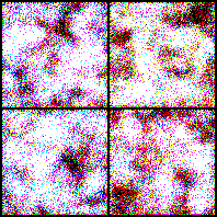
The running results are as follows. It can be seen that there was a lot of noise during the initial training. By the 200th iteration, some outlines could be reconstructed, but the performance was still average. To help everyone understand better, the tutorial did not include many improvement techniques, such as attention mechanisms or class conditional generation. After completing this course, you can continue to learn more~

9.9 Sampling Generation Process

After training ends, the generation phase starts with pure Gaussian noise:

Then, perform a reverse loop according to the time step:

The sample function in the code implements this process:

python@torch.no_grad()
def sample(self, model: nn.Module, shape: tuple[int, int, int, int]) -> torch.Tensor:
    model.eval()
    x = torch.randn(shape, device=self.device)

    for step in reversed(range(self.timesteps)):
        t = torch.full((shape[0],), step, device=self.device, dtype=torch.long)
        pred_noise = model(x, t)
        beta_t = self._extract(self.betas, t, x)
        alpha_t = self._extract(self.alphas, t, x)
        alpha_bar_t = self._extract(self.alpha_bars, t, x)
        mean = (1.0 / torch.sqrt(alpha_t)) * (
            x - beta_t / torch.sqrt(1.0 - alpha_bar_t) * pred_noise
        )
        x = mean if step == 0 else mean + torch.sqrt(beta_t) * torch.randn_like(x)

    return x.clamp(-1, 1)

The reverse mean is:

This line in the code:

pythonx = mean if step == 0 else mean + torch.sqrt(beta_t) * torch.randn_like(x)

Indicates that no additional random noise is added in the last step. Otherwise, the generated $x_0$ will be affected by the last noise perturbation.

9.10 Test Generation Script

generate_stl10_ddpm.py only generates content and no longer reads training data. Its process is as follows:

1. Load checkpoints/stl10_ddpm.pt;
2. Rebuild UNet96 based on base and image_size in the checkpoint;
3. Load model weights;
4. Reverse sample from standard Gaussian noise;
5. Save the generated image.

Core code is:

pythoncheckpoint = torch.load(args.checkpoint, map_location=device)
image_size = int(checkpoint.get("image_size", 96))
model = UNet96(base=int(checkpoint["base"])).to(device)
model.load_state_dict(checkpoint["model_state"])

diffusion = Diffusion(timesteps=int(checkpoint["timesteps"]), device=device)
with torch.no_grad():
    images = diffusion.sample(model, (args.num_samples, 3, image_size, image_size))
    utils.save_image((images + 1) / 2, args.out, nrow=max(1, int(args.num_samples**0.5)))

Example of running mode:

bashpython generate_stl10_ddpm.py --checkpoint checkpoints/stl10_ddpm.pt --out outputs/generated_stl10.png --num-samples 1

Only one sheet is generated by default. $96\times96$ Images are helpful to first check whether the model can actually generate visible structures from noise. If you want to see multiple images, you can increase the scale. --num-samples。

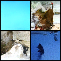
The execution result is as follows:

10. Common Questions

10.1 Is the forward process of DDPM learned?

No. Forward process:

It is a manually defined noise addition rule. What needs to be learned is the reverse process:

10.2 Why No Step-by-Step Noise Addition During Training

Because there is a closed formula:

It can directly obtain $x_0$ to get $x_t$ at any time step.

10.3 Why the goal is to predict noise, not the image

Since the noise during training $\epsilon$ is sampled by us, it naturally serves as a supervised label. After predicting the noise, $x_0$ can be restored using a formula or the reverse mean can be constructed:

Therefore, the prediction noise is not weak; it is equivalent to learning the reverse denoising step.

10.4 What is the biggest difference between DDPM and VAE?

VAE is:

That is, generating an image in one step from latent variables.

DDPM is:

That is, starting from noise, multi-step denoising is performed to generate an image.

10.5 What are the disadvantages of DDPM?

The main drawback is the slow sampling process. It usually requires a step-by-step reverse calculation from $T$ to $1$, and the basic version may require hundreds to thousands of steps. Later, DDIM, an acceleration sampler, or distillation methods can be used to reduce the number of sampling steps.

11. Summary

The core logic of DDPM is:

1. Fixed forward noise addition:

2. Introduce noise at any time:

3. Learn reverse denoising:

4. Obtain the true posterior match using ELBO:

5. Convert the Gaussian KL to mean MSE, and then to noise prediction MSE:

Compared to VAE, DDPM does not compress all image information into a low-dimensional latent variable, but instead removes noise gradually in the image space. Its training objective comes from probability derivation, but it ultimately reduces to a very simple supervised learning problem.

12. After-class Exercises

1. Why is VAE prone to generating blurred images?
2. Why doesn’t DDPM directly generate images from latent variables in one step?
3. What does $\beta_t$ control in the forward process?
4. Why is a square root coefficient used in the one-step noise addition formula?
5. How can $x_t$ at any time step be sampled directly from $x_0$?
6. Why does $x_T$ approach standard Gaussian noise?
7. Why is the reverse process of DDPM modeled as a Gaussian distribution?
8. What constraint does the intermediate KL term in ELBO decomposition impose?
9. Why does the true posterior $q(x_{t-1}|x_t,x_0)$ have an analytical solution?
10. Why is the predicted noise $\epsilon$ equivalent to learning reverse denoising?
11. Why is no noise added in the last step during sampling?
12. What problems will occur for DDPM networks without time embedding?

Appendix A: Detailed Derivation of DDPM ELBO Decomposition

DDPM minimizes negative ELBO:

Expand the model joint distribution:

Expand the forward distribution:

Substitute:

Unpack the log:

Usage for $t>1$:

So:

By substituting these items and organizing the telescoping items, we can obtain:

Written in KL format:

This expression indicates that the core of training DDPM is to make the model’s reverse step distribution match the true posterior derived from the forward process.

Appendix B: Detailed Derivation of the Real Posterior $q(x_{t-1}|x_t,x_0)$

Let:

We require:

According to the Bayes’ formula:

Among them:

Only look at the index part related to $z$:

Expand the first item:

The parts related to $z$ are:

Expand item two:

The parts related to $z$ are:

Merge:

The standard exponential form of the Gaussian distribution is:

Compare the quadratic coefficient:

So:

Normalization:

Because:

And:

So:

Therefore:

i.e.:

Calculate the mean again. From the linear term coefficient: