LEWM World Model Analysis and Interpretation

Is it still confusing after reading the LeWM paper? Are you stuck when reproducing the code due to representation crashes, SIGReg, or high-dimensional normal distributions? Can’t you understand why it is simpler and more stable than JEPA and PLDM?

This article explains the LeWM from start to end in the most straightforward language and clear structure. It helps you fully understand the latest LeWM world model algorithm in one go. It is useful for both getting started with world models and advanced research!

1. First, understand the core problem: What exactly is representation collapse?

The LeWM paper is dedicated to solving the representation collapse problem in world model training throughout its entire content.

Let’s take a simple example to explain the representation collapse problem:

Enter a picture of a car in motion, allowing the world model to infer where the car will be next second, and then output the corresponding feature vector to understand the physical laws in the environment. However, since both the encoder and predictor of the model are trained together, the model tends to take shortcuts. No matter what input image you provide, the encoder outputs a fixed 0 vector. Consequently, when predicting future states, all future states are also 0. This results in a perfect error between the predicted value and the actual value, minimizing the loss function, and the model “wins effortlessly”. When you use this trained model for downstream tasks, it cannot distinguish between different images because all features appear the same to it. This means the model was trained in vain, and the extracted features are completely useless.

This problem is a relatively common one in self-supervised learning. If you try to train the encoder and predictor end-to-end, there is a high chance of encountering this issue.

II. What are the existing solutions? What pitfalls do they hide?

Category 1: External methods that only address symptoms, not the root cause

These issues do not solve them from within the model itself; instead, external methods are used to “patch” the model. The main approaches include:

Heuristic rules: Some rules are established based on experience to restrict the model, such as forcibly constraining the mean and variance of features to not be too extreme. However, the problem is clear: when switching to a different task or dataset, these rules become ineffective, and there is little generalization ability.
Multi-objective loss function: In addition to the main prediction loss, a set of auxiliary losses are added to constrain the features. For example, in the paper mentioned PLDM, 7 loss functions are directly used. However, the weights between these losses need to be adjusted repeatedly. If not adjusted properly, the training curve may become unstable.
Use a pre-trained model directly: For example, DINO-WM. Take the pre-trained DINOv2 visual model that has been trained on large datasets as the encoder. During training, keep the parameters of the encoder fixed without any updates. This indeed ensures stability, as the feature extraction capability is already trained. However, this completely goes against the original purpose of self-supervised learning—learning features from scratch—it is a form of “avoiding problems” rather than solving them. More importantly, the upper limits of the model are locked by the pre-trained model. For instance, when performing robotic arm grasping tasks, the pre-trained model was trained on natural landscape images and has no understanding of the key features in your task. There is no chance to fine-tune it, so you have to replace the pre-trained model, which simply adds a lot of extra work.

Category 2: Internal methods that “work but are hard to explain”

These methods are the approaches used in the JEPA series models (I-JEPA, V-JEPA). For example, Stop-Gradient (SG) + Exponential Moving Average (EMA) is adopted.

SG: The model is divided into two parts. One is the student (online encoder + predictor), and the other is the teacher (target encoder). When the student makes a mistake, only the student is punished, and the student’s parameters are updated. The teacher’s parameters are never touched. This is called stopping gradients. Why do this? If the teacher is allowed to adjust according to the student’s mistakes, in order to get a perfect score from the student, the teacher would change all answers to 0. Both of them would perform poorly together, leading to a breakdown. Cutting off gradients means cutting off the model’s way to take shortcuts. So how are the teacher’s parameters obtained? EMA is used.

EMA: The teacher’s parameter is the slow average of students’ parameters over a certain period. Students learn gradually at the beginning, while the teacher stays steady behind, ensuring that the teacher can set meaningful learning goals for students, and also keeping the teacher’s parameter stable without sudden fluctuations.

This method is indeed effective, and it is widely used now. However, it has a fatal flaw: mathematically, there is no way to explain why it works.

What is the traditional machine learning framework? You have a clear loss function, strictly compute derivatives using calculus during training, calculate gradients, and then update parameters in the direction of gradient descent to find the minimum of the loss. However, in this approach:

Stop the gradient, which means artificially cutting off the gradient flow of backpropagation. The parameters you update are not the actual derivative of the entire system. In EMA, the teacher’s parameter updates are not calculated based on gradients or derivatives; instead, they forcibly use the student’s previous parameters for a weighted average (for example, the teacher’s new parameter = 0.99 × the teacher’s old parameter + 0.01 × the student’s new parameter).

In other words, this is an empirical black-box manipulation. It works, but it is not theoretically sound. Parameter tuning is also extremely complex; even a slight change in a hyperparameter can cause the model to fail directly.

III. The core solution of LeWM: How is the crash problem solved at its root?

Now let’s look at the core innovation of LeWM. It uses a particularly clever method to solve the representation collapse problem when the encoder and predictor are trained simultaneously from the root, and it is supported by a rigorous mathematical theory. Additionally, it is very easy to implement.

First, understand the basic model structure of LeWM

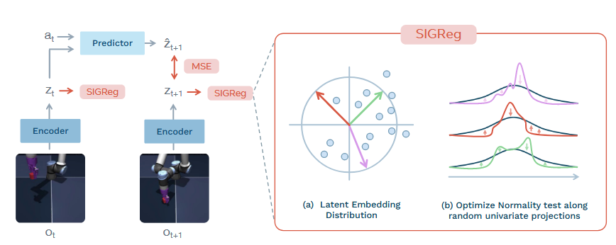
The infrastructure of Leworldmodel is particularly simple, consisting of two core modules: Encoder and Predictor.

\text{Encoder: } \quad z_t = \text{enc}_\theta(o_t)

\text{Predictor: } \quad \hat{z}_{t+1} = \text{pred}_\phi(z_t, a_t)

The encoder uses the Vit architecture. It inputs the environmental image at the current moment $o_t$ , compresses and encodes it into a high-dimensional latent feature vector $z_t$ , and uses this to extract features from the image.
The predictor receives the current features $z_t$ output by the encoder, as well as the action performed by the agent $a_t$ . It predicts the feature representation at the next moment $z_{t+1}$ , allowing the model to simulate how the environment will change in the latent space and understand physical laws.

Then, with the model in place, how is training done? This is the most core innovation of lewm. lewm uses a clever method to solve the problem where, when the encoder and predictor are trained simultaneously, the encoder might lazily map all inputs to a constant vector. As shown in the following code:

python# LeWM loss
output["pred_loss"] = (pred_emb - tgt_emb).pow(2).mean()
output["sigreg_loss"]= self.sigreg(emb.transpose(0, 1))
output["loss"] = output["pred_loss"] + lambd * output["sigreg_loss"]

It can be seen that, compared to PLDM which uses 7 loss functions mentioned in the paper, lewm only uses two loss functions, resulting in an unstable training curve.

pred_loss is easy to understand. The core goal of world model training is to compute the mean squared error between the feature pred_emb predicted by the predictor at the next time step and the feature tgt_emb actually encoded by the encoder at that same time step. The smaller this loss, the better the model’s ability to predict future states and the more accurate its understanding of environmental physical laws.

But with only this loss, the model will surely take a shortcut and suffer a representation collapse. At this point, the core innovation of this paper, SIGReg loss, is needed.

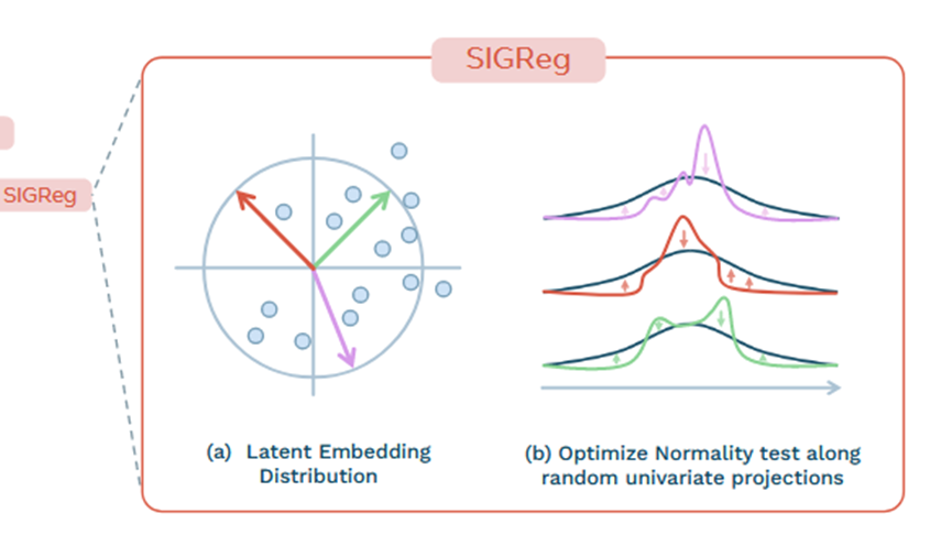
First, as we learned earlier, what is the essence of a collapse? It is when the model maps all inputs into a single constant vector (such as all 0s). In this case, the distribution of features is not a normal distribution at all, but a fixed single point. Conversely, if we could force the model to output high-dimensional features that conform to a perfect high-dimensional normal distribution, it would be impossible for all features to become a single constant, thus eliminating any possibility of taking shortcuts.

However, there is a challenge here: for the normal distribution test of one-dimensional data, there are many established and effective methods, such as the Epps-Pulley test. But for a high-dimensional feature, like the 192-dimensional vector used in the paper, it is very difficult to determine whether it follows a high-dimensional normal distribution.

How does LeWM solve this problem? It uses a particularly clever method: random projection + one-dimensional normality test, which is the SIGReg method.

\text{SIGReg}(Z) \triangleq \frac{1}{M} \sum_{m=1}^{M} T(h^{(m)})

\mathcal{L}_{\text{LeWM}} \triangleq \mathcal{L}_{\text{pred}} + \lambda \text{SIGReg}(Z)

Simply find M different random directions in the d-dimensional feature space, and project all the high-dimensional features onto these M one-dimensional lines. This will yield M sets of one-dimensional feature data. Then, apply the established Epps-Pulley test to each of these M sets of one-dimensional data to ensure they conform to a one-dimensional normal distribution.

Reading papers may be difficult to understand. Here is a very simple example for you:

You want to check if a complex cloud suspended in the air is a perfect sphere (corresponding to a high-dimensional normal distribution). It is too difficult to directly measure its three-dimensional volume and surface curvature. So you use a flashlight and shine it from M random angles on the cloud, then observe the shadows on the wall. If the shadows at each angle are perfect circles (corresponding to a one-dimensional normal distribution), then this cloud is likely a perfect sphere.

LeWM follows this logic. During training, M projection directions are randomly selected, forcing the features to follow a one-dimensional normal distribution in all of them. As training progresses, this is equivalent to shaping the entire high-dimensional feature space into a perfect high-dimensional normal distribution. If the model wants to map all features to 0, it is impossible, as a zero-only distribution cannot pass the normality test, resulting in a high SIGReg loss. The model has no way to take a shortcut.

Most importantly, the entire method is extremely simple. You only need to adjust two hyperparameters: the dimension M of random projection, and the weight lambda between two losses. This greatly simplifies the selection of hyperparameters, allowing beginners to get started quickly.

Meanwhile, there is a mathematical theorem that provides a guarantee for us: the Cramér–Wold theorem. For a high-dimensional data set, if it follows a normal distribution in all possible one-dimensional projections, then this high-dimensional data itself must be a high-dimensional normal distribution.

IV. How to Use the Trained LeWM? How to Drive an Agent with a world model

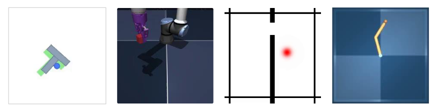
Training the world model is not aimed at making it predict features, but rather to enable it to truly drive agents and complete tasks in the environment, such as robotic navigation and robotic arm grasping. This section aims to explain how a trained LeWM can be implemented into actual executable actions.

The core function of the world model is to predict future states based on current images and actions, then simulate trial-and-error in the mind to find the optimal actions that can achieve the goal. Here, we break down the dense and complex text in the paper into step-by-step processes, making it ten times easier to understand than the description in the paper.

Step 1: Encode the goal and current status first

\hat{z}_1 = \text{enc}_\theta(o_1), \quad z_g = \text{enc}_\theta(o_g)

Using the trained world model encoder, encode the current real image and the final image of the task goal. Compress both images into 192-dimensional latent feature vectors, denoted as $z_1$ and $z_g$ respectively.

The ultimate goal is to find a series of actions that enable the agent to move from the current $z_1$ state to the target state $z_g$ .

Step 2: Try out countless options in your mind to simulate the future trajectory

\hat{z}_{t+1} = \text{pred}_\phi(\hat{z}_t, a_t)

A large number of candidate action sequences are randomly generated. Each sequence includes actions for the next H steps (for example, if H=10, it plans what to do in the next 10 steps).

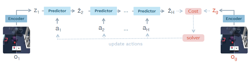
Then, each candidate action sequence is input into the LeWM predictor. Starting from the current state $z_1$ , the first action $a_1$ is combined to generate the next $z_2$ . Then, $a_2$ is combined to produce $z_3$ . In this way, an autoregressive prediction continues until the final state $z_h$ at step H.

The core idea is to use the world model in the potential space to simulate in advance what each set of action plans will result in, without having to test in real-world environments.

Step 3: Filter out optimal actions and iterate for optimization

\mathcal{C}(\hat{z}_H) = \|\hat{z}_H - z_g\|_2^2

a_{1:H}^* = \arg\min_{\boldsymbol{a}_{1:H}} \mathcal{C}(\hat{z}_H),

After simulating all the scenarios, we calculate the gap between the final $z_h$ obtained for each scenario and the target state $z_g$ . The smaller the gap, the better the action, and it helps us complete the task more effectively.

Then we select the top k best-performing solutions. Based on the mean and variance of these excellent solutions, we update the action sampling distribution. Just like evolution, good actions are retained, while poor ones are eliminated. After several iterations, an optimal action sequence is obtained.

Step 4: Take action and see how it goes.

Although the optimal actions for the next H steps are planned, these steps will not be executed all at once. Since the world model’s prediction is autoregressive, each prediction contains a small error. As the number of prediction steps increases, the errors accumulate. If H steps are executed immediately, the agent may move further away from the goal in the end.

5. What are the advantages of LeWM over existing solutions?

After explaining the entire logic, let’s summarize: What makes LeWM better than previous solutions, and why it deserves in-depth study:

Addresses representation collapse at its root with rigorous theory: Unlike the black-box manipulation of SG+EMA, LeWM starts from the essence of feature distribution and is supported by rigorous mathematical theorems, thereby reducing the possibility of the model taking shortcuts.
Very few hyperparameters, and training is simple and stable: Only two hyperparameters, M and lambda, need to be adjusted for the entire model. This is much easier compared to the complex parameter tuning of multi-loss functions and the JEPA series, and the training curve is also particularly smooth.
End-to-end training from scratch, without relying on pre-trained models: There is no need to use a trained large model to freeze the encoder. Instead, a dedicated world model can be trained from zero based on your specific task. The expressive capabilities and upper limits of the model are completely unrestricted, making it highly suitable for niche tasks such as robotics and embodied AI.
The architecture is extremely simple, making it easy to modify and expand: There is no complex teacher-student dual architecture; it is a simple structure of encoder + predictor. It is very convenient to add any module or make improvements.

VI. Current limitations and potential research directions for further exploration

Current Limitations

Adaptation issue of potential space dimensions: The paper uses a 192-dimensional potential space. When dealing with simple tasks that require a very low dimension like tworoom, it may be like using a sledgehammer to crack eggs—it can instead disrupt the natural expression of features and lead to a decline in model performance.
The adaptability to complex real-world environments remains to be verified: Current experiments are mostly conducted in clean and simple simulation environments. However, in real life, there are various disturbances such as lighting changes, obstructions, and dynamic objects. The performance of the model in such complex environments requires further research and validation. For example, increasing the dimension of M can enhance the model’s ability to fit complex features.
Dependence on action labels: Currently, the training of models requires input of action labels for each moment. However, in reality, most video data lacks such labels, which limits the possibility for models to perform pre-training using vast Internet data.

Research directions that can be further explored

Adaptive latent space dimension design: A solution can be designed to automatically adjust the latent space dimension based on task complexity. Simple tasks use a low dimension, while complex tasks use a high dimension, thus avoiding the problem of using an inappropriate tool for a simple task.
Combine inverse dynamics modeling to avoid reliance on action labels: This approach is also mentioned in the paper. Instead of depending on externally provided action labels, a reverse dynamics module can be added to the model, allowing it to infer actions from continuous video sequences. In this way, the model can directly learn general physical laws using unlabeled internet videos, significantly improving its generalization ability.

VII. Guidelines for Reproducing Experiments Without Errors

1. Configure the environment

There are two options. One is the uv management provided by the official source:

pythonuv venv --python=3.10
source .venv/bin/activate
uv pip install stable-worldmodel[train,env]

Another way that everyone can use is to manage with our familiar conda:

pythonconda create -n lewm python=3.10
conda activate lewm
pip install stable-worldmodel[train,env]

2. Download data

Here, we recommend downloading the tworoom and cube datasets. Since the official model weights provided in Google Drive cannot be accessed due to website restrictions, we had to train the tworoom and cube environments from scratch to obtain the weights. Due to limited time and resources, tworoom was trained for a full number of rounds, while cube was only trained for 12 rounds. Those who want to try it can train it by themselves. (The model pt weights provided by the official source on Hugging Face are not the ckpt weights required for evaluation. There is no need to download them, or you can modify the test file to load ckpt instead of pt.)

Download address for the model weights trained by oneself: https://huggingface.co/Datawhale/lewm/tree/main

Tworoom task data address: https://huggingface.co/datasets/quentinll/lewm-tworooms/tree/main

Cube task data address: https://huggingface.co/datasets/quentinll/lewm-cube/tree/main

Pusht task data address: https://huggingface.co/datasets/quentinll/lewm-pusht/tree/main

Reacher task data address: https://huggingface.co/datasets/quentinll/lewm-reacher/tree/main

Create a new folder for each task. For example, the directory structure for the tworoom task is as follows:

pythonlewm
└── tworoom
    └── tworoom
        ├── lewm_object.ckpt
        └── tworoom.h5

Among them, tworoom.h5 is the decompressed data file, and lewm_object.ckpt is the model weight file.

The cube task is a bit different.

pythonlewm
└── cube
    ├── ogbench
    │   └── cube_single_expert.h5
    └── cube
        └── lewm_object.ckpt

Other tasks can set the path by themselves.

3. Training and Testing

First, you need to set the path:

Here, it must be set to a path that includes an extra folder. Otherwise, the model weights will be saved under your lewm, creating a messy situation. This path needs to be loaded for each subsequent step.

pythonexport STABLEWM_HOME=/home/your-user/lewm/tworoom

Training section:

Add your own wandb in config/train/lewm.yaml: https://wandb.ai/home

pythonwandb:
  config:
    entity: your_entity
    project: your_project

Start training:

Fill in the task you want to train after data.

pythonpython train.py data=tworoom

Reasoning Test:

You can use the weights trained by us or the weights trained by yourself. For subsequent task changes, only two places in tworoom need to be modified. Additionally, for distinction purposes, the names of tworoom and cube weights have been renamed during uploading. During testing, the weight names provided by tworoom and cube are placed in the folders of their respective tasks, and then uniformly changed to the name lewm_object.ckpt.

pythonpython eval.py --config-name=tworoom.yaml policy=tworoom/lewm

4. Effect Demonstration

tworoom effect demonstration

python==== RESULTS ====
metrics: {'success_rate': 98.0, 'episode_successes': array([ True,  True,  True, False,  True,  True,  True,  True,  True,
        True,  True,  True,  True,  True,  True,  True,  True,  True,
        True,  True,  True,  True,  True,  True,  True,  True,  True,
        True,  True,  True,  True,  True,  True,  True,  True,  True,
        True,  True,  True,  True,  True,  True,  True,  True,  True,
        True,  True,  True,  True,  True]), 'seeds': None}
evaluation_time: 179.38973236083984 seconds

It can be seen that the success rate of the tworoom simple navigation task is relatively high.

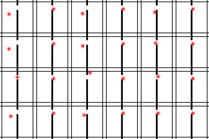
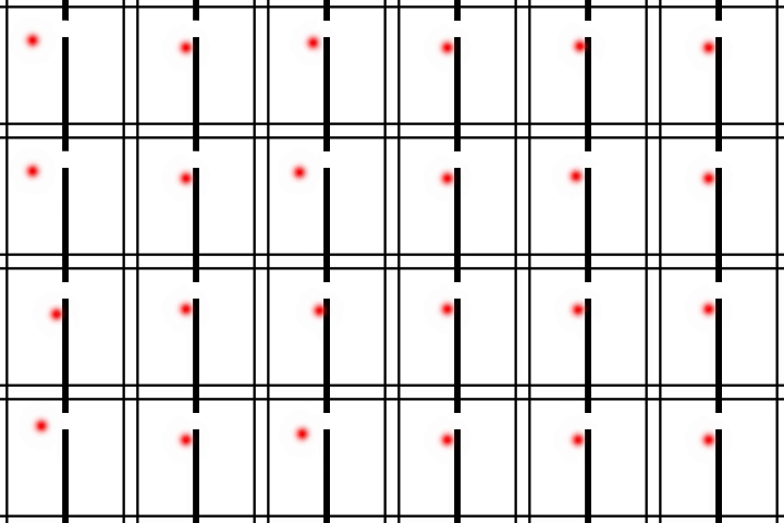
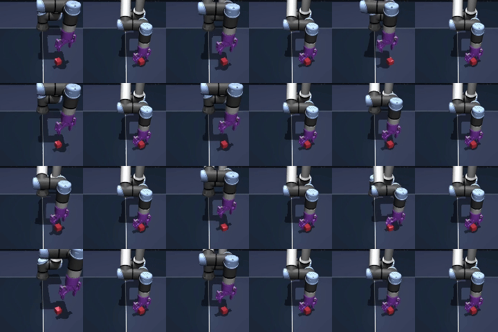
Cube effect demonstration

python
==== RESULTS ====
metrics: {'success_rate': 64.0, 'episode_successes': array([False, False,  True,  True,  True,  True, False,  True,  True,
       False,  True, False,  True,  True, False,  True,  True, False,
        True,  True,  True,  True, False, False, False,  True, False,
       False,  True, False,  True, False,  True,  True,  True,  True,
       False,  True, False,  True,  True,  True, False,  True,  True,
        True, False,  True,  True,  True]), 'seeds': None}
evaluation_time: 191.06767058372498 seconds

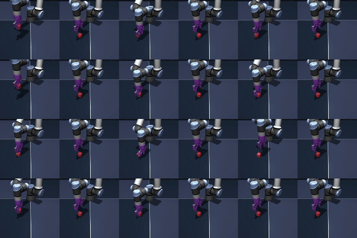
As can be seen, the success rate of the robotic arm grasping task is low. In fact, we believe it may be even lower—possibly due to only 12 rounds of training. We can try training 99 rounds provided by the official source code later. However, the success criteria in the official source code are as follows:

pythondef _compute_successes(self):
    cube_successes = []
    for i in range(self._num_cubes):
        obj_pos = self._data.joint(f'object_joint_{i}').qpos[:3]   # 方块当前位置
        tar_pos = self._data.mocap_pos[self._cube_target_mocap_ids[i]]  # 目标位置

        if np.linalg.norm(obj_pos - tar_pos) <= 0.04:  # 欧氏距离 ≤ 4cm
            cube_successes.append(True)
        else:
            cube_successes.append(False)
    return cube_successes

As long as the block position is correct, it is considered successful. In fact, sometimes the state of the robotic arm also serves as a criterion for determining the success rate, so there may be some deviations.

VIII. Acknowledgments

The content of this article is based on the core ideas of the original LeWM paper. I am grateful for the excellent work of the original authors. I hope this accessible interpretation can help more students who want to get started with world model and embodied AI. Also, I welcome everyone to exchange ideas, share additional reproduction experiences, and propose further optimization strategies.