Introduction to the Mathematical Basis of Diffusion and Problem Analysis

The core issue of the generation model is:

We hope the model learns a data distribution $P_{data}(x)$, and then can sample new samples from this distribution $x$.

For example: facial image distribution, handwritten digit distribution, circular cloud distribution, text, audio, and video distribution, etc.

However, data distributions are usually complex. We cannot directly describe their distribution and density functions, so we need some techniques to solve these problems.

Many people are intimidated by a bunch of formulas when getting started with diffusion models. In fact, the principle of diffusion is quite simple. This content uses simple code to explain the diffusion model, allowing everyone to get familiar with VAE and ddpm without having to derive complex formulas.

In the first part of this chapter, we will explain the mathematical foundations required for diffusion models, which are mainly used for subsequent formula derivations. If you want to directly experience the diffusion model, you can directly refer to the content in the second part. It is a simplified version of VAE and DDPM, providing a complete and simple diffusion experience. In the third part, based on the content in the second part, we explain that some functions in the second part cannot be obtained, which is why we need a diffusion model.

I. Mathematical Foundations

1. Bayesian Formula

When learning about Bayesian formulas, we often see the following form:

The core idea of this formula is: After seeing a result, infer the most likely cause of it.

In tasks such as machine learning, statistical inference, image recognition, and natural language processing, the Bayesian formula is very important. Let’s understand each symbol in the formula one by one.

$z$: Potential causes

$z$ represents the object we want to infer.

It is usually not directly observed, but rather the reason hidden behind the data, hence it is also called hidden variables.

For example: When observing a patient’s symptoms, we want to determine what disease they have.

$x$: Observation data

$x$ indicates the data we have observed.

For example: a set of symptoms. In the Bayesian formula, we infer the underlying cause $z$ based on the observed $x$.

That is to say: $x$ is the result, and $z$ is a possible cause of this result.

$p(x)$: Evidence or marginal likelihood

$p(x)$ represents the total probability of the observed data $x$, also known as evidence or edge likelihood.

For example, if someone shows symptoms such as “fever, cough, and runny nose,” it can be caused by many factors: cold, influenza, allergies, pneumonia, or other diseases.

Therefore, $p(x)$ will consider the probabilities of all possible causes leading to this observation result.

If the possible cause is discrete, it can be written as: $p(x) = \sum_z p(x \mid z)p(z)$

Its main function is to normalize the probabilities, so that the posterior probabilities of all possible causes add up to 1.

$p(z)$: Prior Probability

$p(z)$ refers to our initial judgment on the cause $z$ before seeing the observation data $x$, also known as prior probability.

For example, when determining whether a person has a cold, if it is the flu season, the probability of the cause “cold” occurring is relatively high; if it is not the flu season, the probability may be lower.

Therefore, $p(z)$ can be understood as our judgment of the cause based on prior experience before seeing the evidence.

$p(x \mid z)$: Likelihood

$p(x \mid z)$ represents the probability of observing data $x$ under the condition that the cause $z$ has been identified. It is also known as likelihood.

For example, if someone really has a cold, what is the probability of symptoms such as “fever, cough, and runny nose”?

The relationship here is: $p(\text{症状} \mid \text{感冒})$

It measures whether a certain cause can well explain the phenomenon we observe. If a cause can well explain the observational data, the likelihood is relatively high; otherwise, the likelihood is low.

$p(z \mid x)$: Posterior Probability

$p(z \mid x)$ represents the probability of cause $z$ occurring after data $x$ has been observed. It is also known as posterior probability.

This is what the Bayes’ theorem ultimately aims to achieve.

For example, when we see a person showing symptoms such as “fever, cough, and runny nose,” we want to know the probability that they are really sick: $p(\text{感冒} \mid \text{症状})$

Therefore, posterior probability can be understood as: a re-evaluation of the cause after seeing the result.

The role of the Bayes’ theorem is to combine the prior probability and observation data to obtain the posterior probability.

Bayes’ Theorem:

It can be understood as: Posterior probability = Likelihood × Prior probability ÷ Evidence

That is:

Therefore, the core function of the Bayes’ theorem is: to update our judgment about a cause based on the observed data and existing experience.

2. Jensen’s Inequality

For the concave function $f$, we have:

For convex functions $f$, the following holds:

In machine learning, usually $\log x$ represents $\ln x$ as a concave function, so:

In many models, what we want to maximize is: $\log p(x)$. However, $p(x)$ is often a score:

So:

This thing is usually not easy to optimize directly. Jensen’s inequality can help us construct a lower bound, that is:

$ \log p(x) \geq \text{某个可优化的目标} $

This lower bound is the core of many generative models.

3. Gaussian Distribution

The Gaussian distribution, also known as the normal distribution, is the most commonly used distribution in generative models.

One-dimensional Gaussian distribution

One-dimensional Gaussian distribution is written as:

We can calculate his probability density function below.

We can start with the simplest standard normal distribution:

The density function of the standard normal distribution can be written as:

Here, $C$ is a variable constant. Since $f(x)$ is the probability density function, the normalization condition must be satisfied:

Substitute $f(x)=Ce^{-\frac{x^2}{2}}$:

And the Gaussian integral is:

So: $C\sqrt{2\pi}=1$

Solution:

Therefore, the density function of the standard normal distribution is:

Let the random variable $X$ follow a normal distribution:

For a one-dimensional Gaussian distribution, it can be normalized to a standard normal distribution.

Let:

Then the standard normal density function is:

Because:

So:

According to the density transformation formula for continuous random variables:

Substituting $u=\frac{x-\mu}{\sigma}$, we get:

Continue to substitute the standard normal density function:

Organized:

Therefore, the density function of the normal distribution is:

Among them, $\mu$ is the mean, $\sigma^2$ is the variance, and $\sigma$ is the standard deviation. The mean controls the center of the distribution, while the variance controls the width of the distribution.

Multidimensional Gaussian Distribution

In the embodied domain, images, hidden variables, and 2D points are usually not one-dimensional variables, but multi-dimensional vectors.

Multidimensional Gaussian distribution notation:

The density function is:

Where: $d$ is the dimension, $\mu \in \mathbb{R}^d$ is the mean vector, and $\Sigma \in \mathbb{R}^{d \times d}$ is the covariance matrix.

If the covariance is a unit matrix:

Then it is standard multi-dimensional Gaussian:

4. KL Divergence

KL divergence is used to measure the difference between two probability distributions, and is also commonly referred to as relative entropy.

Assume there are two probability distributions: true distribution: $P$, approximate distribution: $Q$.

Then, the KL divergence from $Q$ to approximately $P$ is defined as:

If it is a continuous random variable, then:

The KL divergence can be understood as: when the true distribution is $P$, but you use $Q$ for encoding or modeling, the average amount of information added is greater.

That is to say: $P$ represents the actual situation, while $Q$ is your model assumption. The smaller the KL divergence, the closer $Q$ is to $P$. If the KL divergence is $0$, it indicates that the two distributions are identical.

Give a simple example

Assumption:

Then:

If natural logarithm is used, the result is approximately:

The relationship between KL divergence and cross-entropy

Cross-entropy is defined as:

Entropy is defined as:

KL divergence satisfies:

Therefore, in machine learning, minimizing cross-entropy is equivalent to minimizing the KL divergence when $P$ is fixed.

Thus, it can be seen that the KL divergence measures: how much information is lost on average when approximating the true distribution $P$ with the distribution $Q$.

II. Generate Basic Introduction Cases

Talking directly about VAE, DDPM, and FM might confuse people. I was also confused when I was learning at first. So, with a simple example, I aim to give everyone a basic understanding of the generation process, which will be very helpful for learning about diffusion models later on. Now, I will explain the basic generation steps using circular distribution. Let’s get started~

This example is ideal for beginners, as the functions, density, and sampling process of the ring are all able to be explicitly constructed. It also introduces the basics based on the generation structures of vae and ddpm. Later on, in the third part of this chapter, we will briefly explain why vae, ddpm, or other diffusion models are necessary.

We will not train any neural network yet, but use handwritten rules to simulate three generation approaches:

1. Direct sampling: Sampling directly from the mathematical definition of the circle.

2. Simulate VAE sampling: First, sample from the latent variable prior, and then generate circular points in one step using the decoder.

3. Simulate DDPM sampling: Start with Gaussian noise and then remove noise step by step until it reaches the circle.

The target distribution is a two-dimensional circle: $x_1^2+x_2^2=R^2$, which is a circle with a radius of $R$.

We want to generate a batch of 2D points:

And these points lie on the circle with radius $R$:

For example, let’s say:

Then the goal is to generate a distribution like this:

text        * * * * *
     *             *
   *                 *
  *                   *
  *                   *
   *                 *
     *             *
        * * * * *

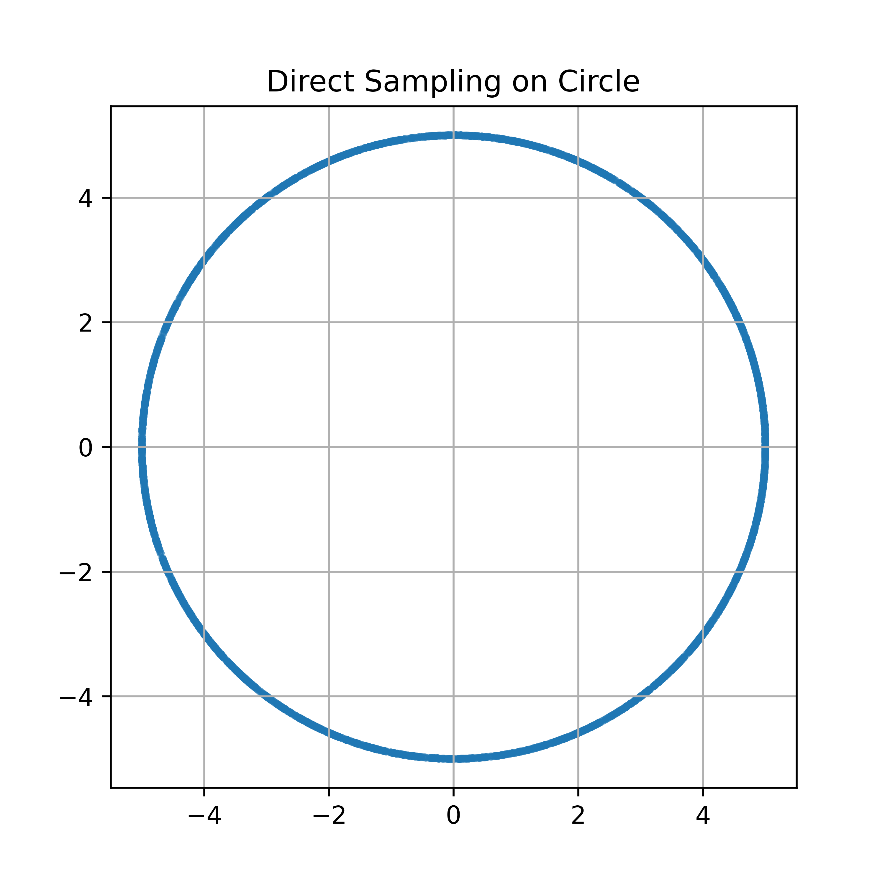
Method 1: Directly sample the circumference

A point on a circle can be parametrized using an angle:

If we want the points to be evenly distributed on the circle, we just need to distribute the angles uniformly:

Then calculate:

This is the most direct circular sampling. As long as you know the explicit form of the target distribution, you can sample directly.

The implementation refers to the direct.py file in the reference code, and the effect is as follows:

Method 2: Simulate VAE sampling around the circle

The generation process of VAE is usually as follows:

The most common prior is the standard normal distribution:

If the decoder is deterministic, it can be simplified to:

In other words, the core generation logic of VAE is: first sample the latent variable z, and then generate x through the decoder.

We can design a handwritten decoder:

Among them:

Then project this 2D Gaussian point onto the circle with radius $R$:

Among them:

Expanded writing is:

The implementation refers to the vae_imitat.py file in the reference code, and the effect is as follows:

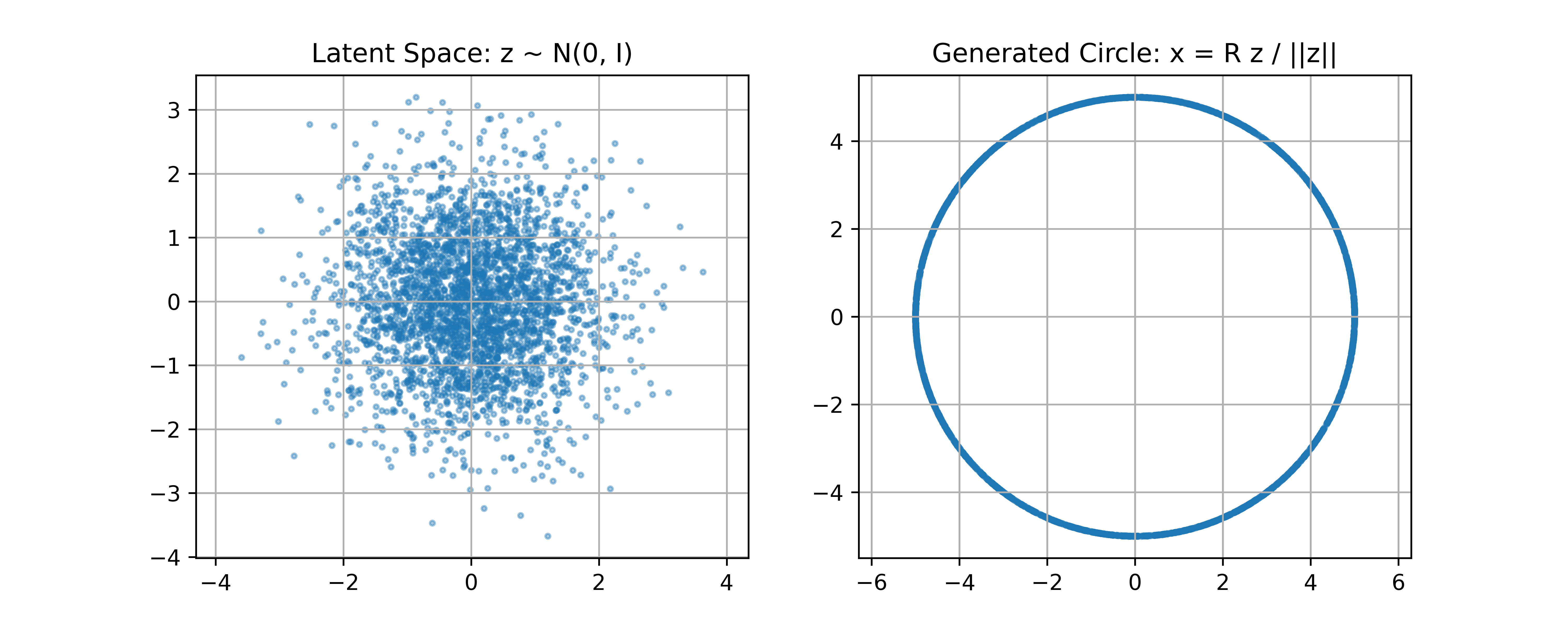
When vae is actually generated, it is produced in one step. This may lead to a biased average result, which is why ddpm is used. This is something that everyone should have a basic understanding of; we will discuss it in detail when we cover vae separately.

Differences between DDPM and VAE

VAE is:

It is generated in one step.

DDPM is:

It is multi-step generation.

Method 3: Simulate DDPM sampling around the circle

The generation of DDPM is not completed in one step.

Its generation process is:

Then, perform noise reduction step by step:

The data samples are finally obtained:

For the circular distribution, the goal is to end up with:

The true DDPM has two processes: 1. Forward noise addition, 2. Reverse denoising.

For beginners, we can first write a manual denoising rule to simulate the sampling process of DDPM.

Core idea is:

1. Start with Gaussian noise.

2. Each prediction should produce a “clean circular point”.

3. The current point approaches the predicted circular point.

4. Add a little more noise at each step, with the noise getting smaller over time.

5. Finally, the point falls near the circumference.

For any current point $x_t$, we can project it onto a circle with radius $R$:

This can be regarded as a handwritten denoising model. In the actual DDPM, $\hat{x}_0$ is predicted by a neural network.

Let the current point be $x_t$. The predicted clean points are:

Then update:

Among them:

Here: $\gamma_t$ controls how close each step gets to the circle, $\sigma_t$ controls how much random noise is added each step. As sampling progresses, $\sigma_t$ should become smaller and smaller.

The implementation refers to the ddpm_imitat.py file in the reference code, and the effect is as follows:

You will see a process:

text标准高斯噪声 -> 点逐渐被推向圆周 -> 最后形成半径为 R 的圆

III. Simplified Parts of the Actual Model

1、VAE

The true VAE is:

Among them, $p_\theta(x|z)$ is the distribution defined by the neural network decoder.

Common forms are:

During sampling:

Among them:

In our simplified version:

Replaced with:

2、DDPM

The forward process of the true DDPM is:

Train neural network:

During sampling, from:

Start and gradually remove noise.

In our simplified version, the neural network prediction is replaced by a geometric projection:

In other words, in the actual DDPM, the neural network learns to denoise x_t into x_0. In our simplified version, we directly project x_t onto a circle using handwriting rules.

In real tasks, we cannot directly obtain distributions that are similar to the circular distribution and can be expressed by mathematical formulas. Therefore, we need to use techniques such as neural network encoding-decoding and re-parameterization to learn the distribution.

How vae, ddpm, and fm specifically learn distributions, generate data, and implement cutting-edge embodied diffusion generation applications such as dreamdojo and dreamzero, as well as other embodied generation technologies like jepa and lewm, will be explained in more detail in subsequent chapters. I hope you gain some insights from this chapter and have a basic understanding of diffusion models.

Thank you all for reading. Fasten your seat belts! Let’s continue to the next chapter~